- VOL 1
- 2026
- research article
Abstract
The equivalent income is a preference-based, interpersonally comparable measure of well-being. Although its theoretical foundations are well established, empirical applications remain limited, primarily due to the detailed data requirements on individuals’ preferences across various well-being dimensions. This paper reviews the literature on preference elicitation methods with a focus on estimating equivalent income. We examine several survey-based methods, including contingent valuation, multiattribute choice or rating experiments, and life satisfaction regressions. The review highlights the advantages and limitations of each method, emphasizing the considerable scope for methodological improvements and innovations.
Introduction
It is now widely recognized that individual well-being is a multidimensional concept that cannot be fully captured by income alone (Stiglitz et al., 2009). Nevertheless, there remains considerable debate about what constitutes well-being and how best to measure it. Several approaches have been proposed (Fleurbaey and Blanchet, 2013). Preference-based measures of well-being build on the principle of individual sovereignty, which asserts that individuals are best positioned to assess their own well-being. More specifically, individual preferences can inform policymakers about what constitutes well-being and provide a basis for measuring it.
Equivalent income is one such measure that respects individuals’ (ordinal) preferences. The equivalent income is the hypothetical income level that, when combined with the reference levels for all nonmonetary dimensions, places the individual in a situation they regard as equally good as their actual situation (Fleurbaey, 2009; Fleurbaey and Blanchet, 2013; Decancq et al., 2015a,b). Typically, the reference levels are set to reflect the best or “ideal” outcomes in the nonmonetary dimensions (Fleurbaey and Blanchet, 2013). The gap between an individual’s actual and equivalent income captures the well-being loss from not attaining these reference levels, expressed in terms of willingness to pay (WTP). Given the choice of the reference levels, the equivalent income provides a cardinal and interpersonally comparable measure of well-being that can be applied in social welfare analysis (Decancq et al., 2015b, p. 94).
To compute the equivalent income, information on individuals’ preferences across various dimensions of well-being is necessary. For dimensions where individuals have the ability to make choices, preferences can be inferred from observed behavior, known as revealed preferences. In the context of equivalent incomes, revealed preference data have been used to capture preferences for life expectancy (Fleurbaey and Gaulier, 2009; Boarini et al., 2022) and labor market outcomes (Bargain et al., 2013; Decoster and Haan, 2015). However, the revealed preference method depends on strong assumptions about choices, including perfect information, the absence of market constraints, and freedom from behavioral distortions (Hausman, 2011). However, its main limitation is that there are many dimensions of well-being over which individuals do not exert choice (such as their health).
To address these challenges, welfare economists are increasingly exploring alternative methods for eliciting preferences. Stated preference methods offer a well-established means to elicit individuals’ WTP or willingness to accept (WTA) for changes across various dimensions. This survey-based approach can be applied to nearly any context, offering a significant advantage over revealed preference methods. Several studies have applied stated preference methods to calculate equivalent incomes, particularly in areas such as income and health (Fleurbaey et al., 2013; Decancq and Nys, 2021). However, the hypothetical nature of stated preference surveys has raised questions about their validity. Simply put, there are numerous reasons why individuals’ stated preferences might differ from their actual behavior in real-life situations, an issue known as hypothetical bias. Additionally, responses can be influenced by subtle aspects of survey design, leading to well-documented biases such as framing and anchoring effects. Stated preference studies are also resource-intensive in terms of time and cost.
An alternative method is to use self-reported life satisfaction data to infer individuals’ preferences. In this method, researchers typically analyze life satisfaction scores by regressing them on income and nonmonetary dimensions of well-being, controlling for sociodemographic factors. The resulting coefficients can then be used to determine the marginal rate of substitution between income and the selected nonmonetary dimensions, which yields the WTP for obtaining the reference level in the nonmonetary dimensions. This method has been used to compute the equivalent income across a variety of dimensions (see, e.g., Decancq et al., 2015a; Decancq and Neumann, 2016; Decancq and Schokkaert, 2016; Jara and Schokkaert, 2017; Murtin et al., 2017). Also this method has limitations, in particular because the coefficient estimations may be biased (due, e.g., to missing variables, reverse causality, or measurement errors).
The aim of this paper is to review various stated preference methods and the life satisfaction approach to evaluate their suitability for estimating equivalent incomes. We focus thereby on two sets of evaluation criteria.
First, we examine the reliability and validity of different methods. Reliability has various interpretations in the valuation literature. Broadly, it refers to the degree of variability (or noise) associated with repeated applications of a valuation method (Bishop and Boyle, 2019). If we assume that preferences are stable over time, a more reliable method yields consistent results upon retrial. The concept of reliability can also be extended to encompass the sensitivity of estimates to small changes in survey design (Rakotonarivo et al., 2016). Validity can be assessed in several ways, commonly referred to as “the three Cs.” Construct validity examines whether the elicited WTP estimates align with prior theoretical expectations. Convergent validity occurs when different methods yield similar estimates of WTP. Criterion validity means the WTP estimate is close to some benchmark value believed to be “true.” However, there is some debate as to whether criterion validity is simply another form of convergent validity (Johnston et al., 2017). In this paper, we focus therefore on construct and convergent validity.
The second set of evaluation criteria addresses the scope of each method. The scope of a method depends on the researcher’s theoretical objectives and the desired degree of preference heterogeneity. It is helpful to distinguish among three theoretical objectives, ranked from least to most ambitious:
-
Measurement of equivalent income. The most direct objective is to estimate well-being itself, with limited attention to trade-offs across dimensions. Contingent valuation methods, for instance, can be used to elicit respondents’ equivalent income by asking them to state their WTP for attaining the reference levels in the nonmonetary dimensions of well-being. The equivalent income is then derived by subtracting this WTP from actual income.
-
Estimation of marginal rates of substitution. A more ambitious objective is to estimate marginal (or nonmarginal) rates of substitution between dimensions of well-being. Researchers may, for example, estimate the WTP for incremental changes in health or other nonmonetary dimensions. Once all marginal rates of substitution are known, the WTP for reaching the reference levels is also derived, and hence the equivalent income.
-
Mapping of indifference curves. The most comprehensive objective is to recover an individual’s full indifference map, or at least those indifference curves (or sets) that are relevant for well-being measurement. Once the indifference curves are mapped, the marginal rates of substitution and, consequently, the equivalent income can also be derived.
Regarding the degree of preference heterogeneity that can be estimated with any given method, we differentiate between methods that aim to capture variations at the individual level and those that aim to capture heterogeneity only at the sociodemographic group level. Although the former methods typically employ nonparametric approaches in the analysis, the latter mainly rely on parametric models in which heterogeneity is introduced through interactions between the parameters of interest and sociodemographic variables. As we will illustrate, the degree of heterogeneity that a method can accommodate is closely related to its theoretical objective. For example, while contingent valuation methods enable efficient estimation of well-being levels at the individual level, they are less suited to estimating marginal rates of substitution or indifference maps. In contrast, multi-attribute methods efficiently estimate these concepts but generally permit only group-level heterogeneity in preferences.
There exists already a large literature on the advantages and disadvantages of different stated preference methods for estimating WTP (see, e.g., Bateman et al., 2002). The empirical literature on estimating equivalent incomes is smaller but growing. Alongside evaluating different preference elicitation methods for the purpose of estimating equivalent incomes, we also provide the first review of this emerging empirical literature. We assess the findings of, and challenges faced by, these studies as well as prospective ways forward. We believe that the insights from this review are valuable not only to those working with equivalent income but also to researchers working on the estimation of WTP or well-being measurement more broadly.
The structure of this paper is as follows. Section 2 reviews the concept of equivalent income. Section 3 categorizes and summarizes different preference elicitation methods. We then provide detailed assessments of the main methods: contingent valuation, including the recent ABDC extension (section 4), multiattribute choice and rating methods (section 5), and the life satisfaction method (section 6). Section 7 evaluates these methods, focusing on theoretical objectives of reliability, validity, and scope, and the level of preference heterogeneity captured. Section 8 reviews empirical evidence on equivalent incomes. Section 9 discusses specific challenges in applying stated preference and life satisfaction methods for equivalent income estimation and presents avenues for future research. Section 10 concludes.
The equivalent income and preference-based approaches
Let the actual life situation of an individual be described by where represents their income and is a vector encompassing nonmonetary dimensions. Let represent the individual-specific vector of reference levels for the nonmonetary dimensions.
Each individual has their own preferences over life situations, which can be expressed as a binary relation . We write to indicate that individual regards to be at least as good as . Indifference and strict preference relations are denoted and , respectively. Preferences are assumed to satisfy the following assumptions. First, we assume that preferences are transitive: if and , then . For mathematical convenience, preferences are also assumed to be continuous, meaning that the upper contour set and the lower contour set are closed. Third, most applications assume complete preferences, meaning that for any pair and , either or (or both) holds. This completeness assumption can be relaxed, with equivalent income then estimated as a range, defined by upper and lower bounds (see Fleurbaey and Schokkaert, 2013). Finally, we assume preferences are monotonic, meaning that whenever is at least as high as in every dimension. This assumption excludes the possibility of satiation, though the concept of equivalent income can also be applied to nonmonotonic preferences, as will be discussed in section 9.
The equivalent income of individual is determined by solving the following equation:
where and denotes the individual’s WTP to attain the reference levels of the nonmonetary dimensions. In other words, equivalent income is the hypothetical income level, , that, when combined with the reference levels for all nonmonetary dimensions, places the individual in a situation they regard as equally good as their actual situation. This well-being measure respects the individual’s conception of a good life. Moreover, it enables interpersonal comparisons of well-being, conditional on the chosen reference levels, by translating each individual’s -dimensional life situation into a single cardinal index consistent with their ordinal preferences.
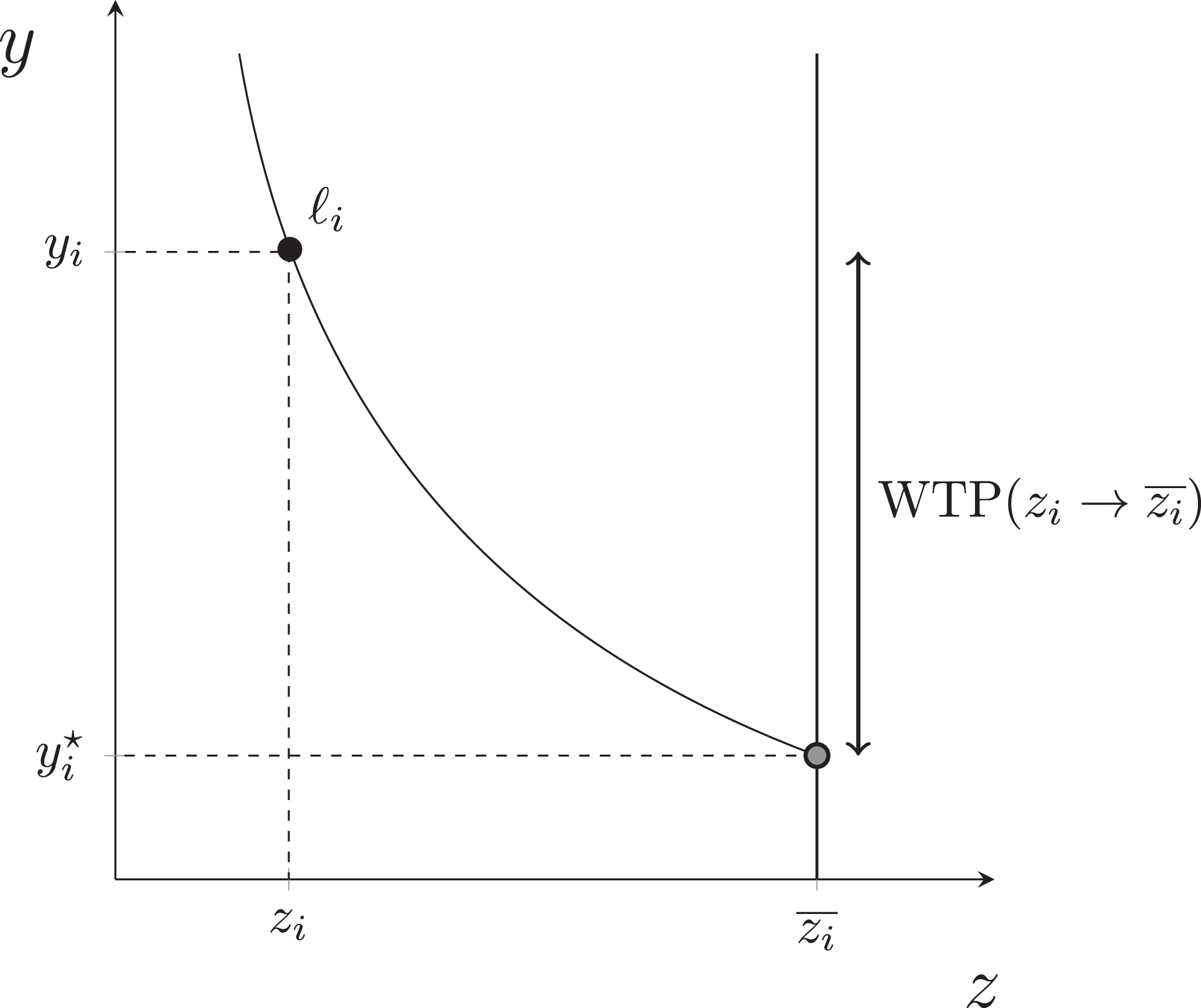
Figure 1 demonstrates the concept of the equivalent income graphically using an indifference curve defined over a two-dimensional space. This curve represents all the combinations of income and the nonmonetary dimensions , which are considered to be equally good by individual according to their preferences. The individual’s actual situation lies on the same indifference curve as the hypothetical situation , indicating that they are indifferent between these two situations, i.e., . Furthermore, the equivalent income is equal to individual ’s actual income level minus their WTP to attain the reference level , which is denoted by the vertical distance WTP .
The concept of equivalent income
The concept of equivalent income
Determining the value of the reference levels is an ethical matter, rather than an empirical one. Ethical arguments support selecting an “ideal” situation across various dimensions as the reference (see, e.g., Fleurbaey and Blanchet, 2013). For dimensions in which there is no satiation and a natural upper bound, the ideal situation is common to all individuals (e.g., perfect health in the health dimension). The choice of the natural upper bound is most prevalent in the empirical literature on equivalent incomes, see section 8. However, when preferences are nonmonotonic and vary across individuals, an alternative is to set an individual-specific reference level that reflects the ideal situation according to individual ’s preferences. In the rest of this paper, we set aside the ethical considerations involved in choosing reference levels and focus on the empirical challenge of estimating preferences.
A taxonomy of preference elicitation methods
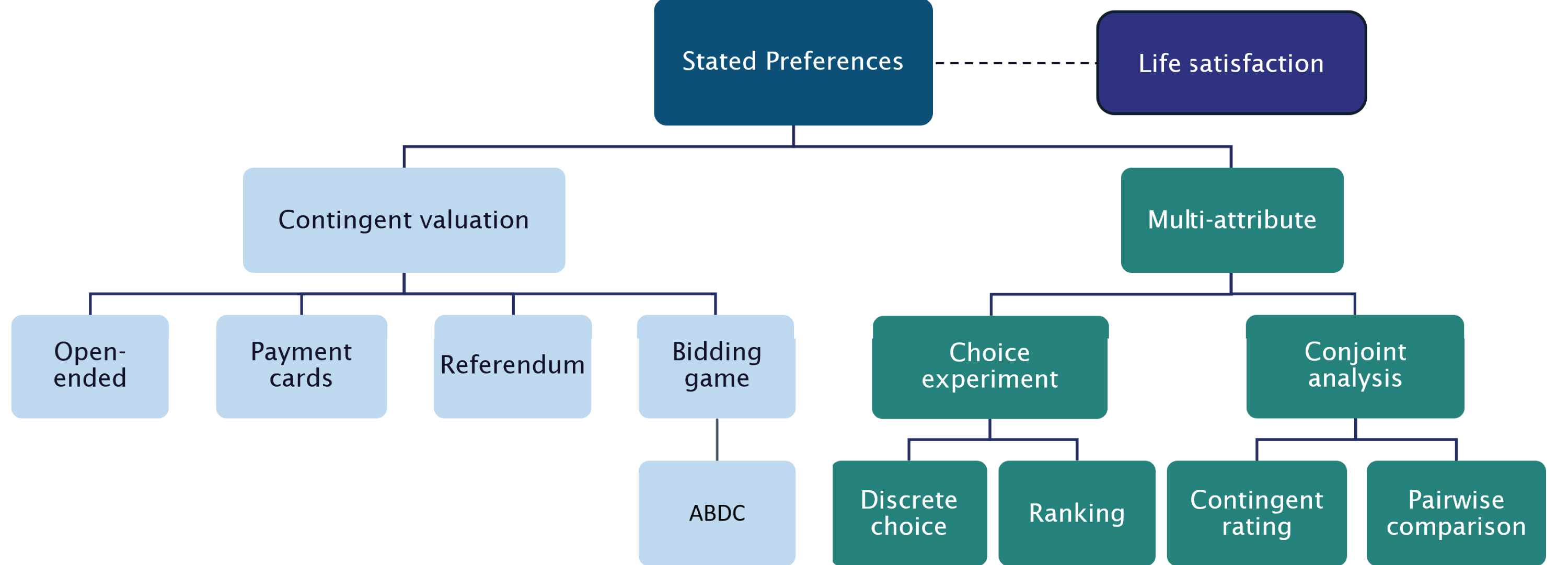
The existing preference elicitation methods can be organized into three broad categories: contingent valuation, multiattribute, and life satisfaction methods. Figure 2 illustrates a taxonomy of preference elicitation methods based on these three categories.
A taxonomy of preference elicitation methods.
A taxonomy of preference elicitation methods.
Contingent valuation is a direct survey method that asks individuals to state their WTP for a change, or a set of changes, in the provision of a nonmarket good, typically treated as a unified whole. For example, in the context of estimating equivalent income, respondents may be asked how much income they would be willing to forgo in order to attain the “ideal” reference levels in the nonmonetary well-being dimensions. This directly measures their equivalent income. The contingent valuation method employs various elicitation mechanisms to estimate WTP, including open-ended questions, payment cards, referenda, and bidding games, all of which are discussed in further detail in section 4.
Multiattribute methods define the changes to be valued as a function of different attributes (e.g., dimensions of life) and their levels (e.g., good health), rather than as a unified whole. By experimentally varying the levels of these dimensions, the marginal WTP for changes in each attribute can be elicited. These methods can be further subdivided into choice experiment and conjoint analysis methods. The former includes discrete choice and ranking experiments, which ask individuals to choose between or rank a set of two or more alternatives. These methods are typically grounded in random utility theory (McFadden et al., 1973), which models individual choice behavior as composed of two parts: a deterministic component (i.e., based on observable factors) and a stochastic error term. Conjoint analysis methods ask individuals to rate an alternative using a predetermined scale (contingent rating) or to indicate their strength of preference for one alternative over another (pairwise comparison). These methods typically utilise deterministic utility functions to model responses, the parameters of which are estimated using linear regression. Thus, conjoint analysis often relies on strong cardinality assumptions due to the use of the scale.
A relatively recent strand of the literature uses self-reported life satisfaction scores to recover information about ordinal preferences. These preferences can be used to construct measures of well-being (e.g., Decancq et al., 2015a) or to value different non-market goods (e.g., Clark and Oswald, 2002; Oswald and Powdthavee, 2008). Typically, researchers regress life satisfaction scores on income and nonmonetary dimensions, while controlling for other socioeconomic and psychological factors. The estimated coefficients are then used to derive the marginal rate of substitution between income and the nonmonetary dimensions. This method combines elements of both revealed and stated preference studies: WTP values are recovered (rather than directly stated) from individuals’ subjective reports of their well-being. Therefore we place this method outside of the contingent valuation and multi-attribute methods in Figure 2.
Before discussing these methods and their advantages and disadvantages in more detail in the following sections, we briefly review some limitations that apply to all reviewed preference elicitation methods:
-
Hypothetical bias: There are several reasons why an individual’s answers in a stated preference survey may differ from their actual behavior in the described scenario. These include: i) a failure to consider budget constraints or substitutes when stating their WTP for a change in a nonmarket good; ii) a desire to please the interviewer by providing the “right” or socially acceptable answer, a problem known as the interviewer effect, that is related to the so-called warm glow effect; or iii) a failure to take the task seriously, leading to trivial responses. It is important to note, however, that actual behavior does not always reflect “true” preferences, particularly in contexts of imperfect information and behavioral biases. Furthermore, individuals often have little or no control over some life dimensions that are crucial to their well-being (e.g., health).
-
Strategic behavior: Certain formats, such as open-ended contingent valuation questions, may be vulnerable to strategic under- or overstatement of the WTP. For example, individuals might overstate their WTP to influence the provision of a public good if they believe that the payment is nonbinding and that free-riding is possible. Carson and Groves (2007) argue that the truthful revelation of preferences depends on whether the survey is incentive-compatible and consequential. Incentive compatibility refers to whether respondents have an incentive to report truthfully, while a consequential survey is one that respondents perceive as having outcomes that could alter the behavior of the issuing agency or impact their own well-being.
-
Protest votes: Respondents may claim not to be willing to pay for a good, even if they value it, due to various reasons such as rejecting the notion of making payments or believing that others should bear the cost.
-
Inconsistent preferences: Several studies have documented inconsistencies in individuals’ preferences when answering stated preference questions. The most frequently cited issues are embedding or scoping effects in contingent valuation research (Hausman, 2012). This refers to situations where WTP does not rise with an increase in the amount of the nonmarket good offered, despite no clear reason for preferences to be nonmonotonic. Arrow et al. (1993) argue that demonstrating scope effects is a key validity test for contingent valuation estimates. While many studies pass scope tests, there remains debate over whether the effects are sufficiently large or plausible (as discussed in section 4.4). Additionally, there is an ongoing debate in the literature over the difference between estimates of WTP and WTA (Haab et al., 2013).
-
Survey design: Stated preference methods are also subject to several biases inherent in survey design, such as question framing and sequence effects when valuing multiple goods. It is also challenging to assess whether respondents fully understand and internalise the information they are asked to consider when making valuations. The validity of estimates can be undermined, for example, if respondents interpret aspects of the good differently or use heuristics to “fill in the gaps” where information is incomplete (Johnston et al., 2017). Moreover, respondents may reject the information presented to them if they believe the costs of a hypothetical government project are overstated. In such cases, respondents may be answering a different question than intended, undermining the validity of the estimates (Arrow et al., 1993).
Contingent valuation method
Contingent valuation data
The contingent valuation method employs a direct survey question to collect the data required to compute equivalent incomes, i.e., the individual WTPs to attain the reference levels in the nonincome dimensions.
Respondents are first presented with a description of a hypothetical situation. In the context of estimating equivalent incomes this consists of a description of a hypothetical life situation in which the nonincome dimensions are fixed at their reference values (see section 4.5 for an illustration).
They are then asked to state their maximum WTP (or minimum WTA) for a change to that hypothetical situation, using a specified elicitation mechanism. Several alternatives are common in the literature. Open-ended questions directly ask respondents to state their WTP for the change. The single-bounded referendum method presents respondents with a (randomly assigned) payment amount and asks whether they would be willing to pay that amount, with a dichotomous choice (yes/no) response. The double-bounded version follows up with a second question to estimate bounds around an individual’s WTP, improving statistical efficiency. In the bidding game, respondents are given multiple rounds of dichotomous choices, with the final question typically open-ended. Under the payment card method, respondents select the value closest to their WTP from a predefined list. Table 1 summarizes these methods and provides examples.
| Mechanism | Example | Advantages | Disadvantages |
|---|---|---|---|
| Open-ended | • What is the maximum amount of income you would give up to obtain ? | • Straightforward question. • Avoids cues (no starting point/anchoring bias). • Provides WTP estimate for each respondent. |
• Large nonresponse rates (protest answers, zeros, outliers). • Cognitively challenging for respondents. |
| Payment card | • What is the maximum amount of income you would give up to obtain ? €0-10, €0-20,…, >€200? | • Avoids starting point bias (cards are laid before respondent). • Number of outliers (i.e., very large bids) may be reduced. • Provides interval coded WTP values at individual level. |
• Responses coded on an interval. • The width of the intervals and limits for the payment cards may lead to potential bias. |
| Referendum | • Single bounded: would you be willing to pay to obtain ? Yes/No • Double bounded: would you be willing to pay to obtain ? (e.g., if Yes, would you pay ; if No, would you pay ?) |
• Cognitively easier for respondents than open-ended. Only one value to consider. • Provides incentives for truthfully revealing preferences. • Minimizes non-response and outliers. • Provides interval coded WTP values at individual level. |
• Vulnerable to “yes-saying” (i.e., giving false affirmative answers). • Subject to starting point bias (i.e., WTP may be influenced by starting bid). • Statistically inefficient as each respondent is only asked one question or two questions (double bounded). |
| Bidding game | • Would you be willing to pay to obtain ? If Yes: interviewer keeps increasing bids until the respondent answers no. If No: interviewer keeps decreasing bids until respondent answers yes. | • Cognitively easier for respondents than open-ended. • Provides single or interval coded WTP values at the individual level. |
• Vulnerable to “yes-saying” (i.e., giving false affirmative answers). • Subject to anchoring bias (i.e., WTP may be influenced by starting bid). |
Finally, contingent valuation surveys usually include debriefing questions to verify respondents’ understanding of the hypothetical situation and assess the validity of the stated valuations.
Estimation of WTP
Nonparametric and parametric estimation techniques can be employed to analyze the elicited contingent valuation data. Open-ended questions and the bidding game (with a final open-ended question) provide individual WTP values directly, which can then be used to compute equivalent income (see section 4.5). Standard linear regression techniques may also be applied to assess the determinants of the elicited WTP values.
Other mechanisms yield binary or interval-coded responses that can be treated as limited dependent variables in interval regression models, which are based on random utility theory (McFadden et al., 1973). Two approaches are commonly used to analyze binary choice data from single-bounded referendum designs. The first is the utility difference model of Hanemann (1984), which uses a random utility model to monetize the utility change. The second is the bid-function model, which directly specifies a functional form for respondents’ WTP.
Since random utility models are discussed in the next section, we illustrate here how the bid-function can be employed to estimate WTP. Let if the individual answers “yes”, and if the individual answers “no” to a randomly assigned bid amount in the referendum survey. The WTP function for a sample can be recovered by specifying the probability that an individual gives an affirmative response to the bid amount as:
where is a function that depends on a set of observed characteristics , such as nonmonetary dimensions of well-being (and possibly also personal characteristics of the respondent), and an error term . By specifying this function as linear in parameters , we obtain:
Assuming different distributions for the unobserved factors leads to various econometric models. For instance, assuming , i.e., that follows a normal distribution, yields an expression close to the standard probit model:
where denotes the standard normal cumulative distribution function. The parameters and can be estimated using maximum likelihood. The estimation of preferences for the double-bounded referendum method extends this approach to the case of interval data (see Hanemann et al., 1991).
Advantages and disadvantages of the contingent valuation method
A key advantage of the contingent valuation method for estimating equivalent incomes is that it provides a direct measure of WTP at the individual level. This is particularly useful when studying how WTP values vary across different individuals. The contingent valuation method is also flexible enough to value a wide range of goods, including those that are considered as an indivisible whole and cannot readily be valued as a function of multiple attributes (Johnston et al., 2017). Some elicitation mechanisms, such as the bidding game or referendum method, mimic familiar, real-world valuation mechanisms, which reduces the cognitive burden on respondents and may enhance the validity of the estimates. Finally, the method is relatively easy to administer and understand. This applies particularly to elicitation mechanisms like open-ended questions and payment cards, which do not require complex experimental designs. The ease of understanding enhances respondent engagement, potentially increasing the credibility of the WTP estimates.
The popularity of different elicitation mechanisms has evolved over the years in response to the advantages and disadvantages of each approach, some of which are listed in Table 1. Early studies relied on an open-ended question, which is by far the most straightforward approach and has the advantage of yielding individual-level WTP estimates. However, this method has become less popular over time due to the difficulty of answering open-ended questions and hypothetical and strategic biases that might arise, leading to implausibly high WTP values or large numbers of protest votes. More recent studies have opted for the referendum method, which mitigates these issues to some extent. The method became particularly popular following the endorsement of the National Oceanic and Atmospheric Administration (NOAA) panel of experts, chaired by Kenneth Arrow and Robert Solow, which highlighted that the single-bounded method reduces strategic bias, by providing incentives for respondents to answer truthfully (Arrow et al., 1993). Carson and Groves (2007) caution that this is only the case if the referendum is single-bounded and perceived by the respondent as consequential. Yet, the core limitation of the single-bounded referendum approach is that it provides very limited information about an individual’s preferences. It may also be subject to anchoring (or starting point) bias, whereby individuals interpret the bid amount as providing information on what is reasonable or expected. The bidding game approach is one alternative that provides more information on preferences by narrowing down the bounds around an individual’s WTP and is cognitively easier than the standard open-ended question. Still, the method is subject to starting point bias as well as the phenomenon of “yes-saying” (i.e., false affirmative answers). Payment cards avoid the latter by providing individuals with a visual set of payment options to choose from. However, the intervals between the payment cards, their position, and the upper and lower limits may still lead to some degree of bias (Hausman, 2012).
Some studies have used variations of contingent valuation designs to reduce such biases. Chanel et al. (2017), for instance, experiment with a circular payment card wheel. Respondents are first asked to think about their maximum WTP and then presented with a pie chart wheel that has different segments with payment amounts. Respondents then move the wheel until they find a section that matches their valuation. Chanel et al. (2017) argue that this format reduces starting point bias as each segment is equally likely to be seen first, and reduces middle-point bias because there is no predetermined start or end points on the wheel. Champonnois et al. (2018) find that this format reduces anchoring bias in a multiple elicitation format. Others have introduced formats that incorporate respondent uncertainty to avoid the problem of “yes-saying.” For instance, Dubourg and Loomes (1997) ask using a disc that they rotate back and forth between different values to elicit the largest amounts the respondent would definitely pay and smallest amounts they would definitely not pay. Welsh and Poe (1998) propose multiple response options to payment card questions ranging from: “Definitely no,” “Probably no,” “Not sure,” “Probably yes,” and “Definitely yes.” Wang and Whittington (2005) introduce a stochastic payment card mechanism in which respondents can state their likelihood to pay different amounts on a numeric scale (0%, 25%, 50%, 75%, and 100%).
Reliability and validity of the contingent valuation method
There has been a long-running debate among economists regarding the validity of WTP estimates derived from contingent valuation studies. This debate was mainly centred on the evaluation of environmental damages. The contingent valuation method initially gained some form of legitimacy after the NOAA panel of experts, concluded that, given a set of best practices, contingent valuation studies “convey useful information” and could provide “estimates reliable enough to be the starting point of a judicial process of damage assessment” (Arrow et al., 1993, p. 43). However, Portney (1994), a member of the panel, notes that this conclusion was made reluctantly, which motivated the panel members to construct a set of best-practice guidelines for future contingent valuation studies. These included stipulations that researchers should: i) use personal instead of mail interviews; ii) elicit WTP instead of WTA; iii) utilize the referendum format; iv) accurately describe the valuation scenario; iv) remind respondents of their budget constraints and substitutes for the good in question; and v) include follow-up questions to measure respondent understanding. Since the NOAA report, economists have remained divided on the validity of the contingent valuation method. Notable examples are provided in two symposia of the Journal of Economic Perspectives in 1994 and 2012, which featured articles from prominent proponents and critics of the contingent valuation method. Generally, proponents argue that when contingent valuation methods are carefully applied they provide meaningful measures of value (see Kling et al., 2012; Carson, 2012). Critics, in contrast, contend that the method is subject to numerous biases and inconsistencies that cast doubt on the elicited WTP values (see Hausman, 2012). While the debate is far from settled, it is important to consider the weight of empirical evidence concerning the validity of the approach and the consequences for the elicitation of equivalent incomes.
Various studies have attempted to assess criterion or convergent validity by comparing estimates from stated and actual scenarios (i.e., using real money payments). Differences are typically interpreted as evidence of hypothetical bias. Existing evidence, principally from the field of environmental economics, suggests that contingent valuation estimates of WTP are generally upwardly biased (List and Gallet, 2001; Murphy et al., 2005; Kling et al., 2012; Hausman, 2012). For instance, the most recent meta-analyses suggest that the mean and median ratio of stated to actual values across studies is around 2 and 1.4, respectively (Foster and Burrows, 2017; Penn and Hu, 2018). However, these findings are not always consistent across fields. In the field of health economics, stated preference estimates of the value of statistical life, i.e., the marginal rate of substitution between income and mortality risk, are typically lower than those derived from revealed preference studies (Alberini, 2019). For instance, Viscusi and Masterman (2017) report a mean value of statistical life of $13.5 million from their meta-analysis of 953 revealed preference studies. In a follow-up review of stated preference estimates, they report an average value of $10.3 million (Masterman and Viscusi, 2018). It remains an open question how the discrepancies between the results in different fields can be explained.
The existence of hypothetical bias has been the subject of considerable debate, particularly regarding whether it reflects the nature of the question or rational responses to the incentives embedded in surveys. Several authors argue that interpreting hypothetical bias from meta-analyses is difficult without considering the incentive structure and the consequentiality of the surveys (Carson and Groves, 2007; Kling et al., 2012; Haab et al., 2013). Carson and Groves (2007) argue that what is often perceived as hypothetical bias may actually be a rational response to the incentives present in the survey design. For example, they note that referendum surveys for hypothetical public goods may incentivize respondents to overstate their WTP if they believe that a government agency will not be able to enforce payment if the good is provided. In this regard, Carson and Groves (2007) assert that only incentive-compatible and consequential surveys can reliably predict how rational agents will respond. Haab et al. (2013) further observes that several studies meeting these criteria have shown no evidence of hypothetical bias.
Various ex ante survey methods have been developed to mitigate different forms of hypothetical bias in contingent valuation (see Loomis, 2011). One common approach, known as cheap talk, involves reminding respondents of the tendency to overstate values before they answer the contingent valuation question (see Cummings and Taylor, 1999). Budget reminders ask respondents to consider their budget constraints when stating their WTP, while honesty oaths require respondents to pledge truthfulness prior to answering (see Jacquemet et al., 2013). Another method, consequentiality scripts, emphasizes the potential importance of their responses, particularly in relation to policy changes that may affect their personal well-being. Evidence on the effectiveness of these approaches is mixed, with some studies finding limited reductions in hypothetical bias and improvements in validity (Johnston et al., 2017). Recent meta-analyses suggest that methods like cheap talk, consequentiality scripts, and uncertainty analysis may reduce hypothetical bias to a degree, though generally by only a small margin (Foster and Burrows, 2017; Penn and Hu, 2018).
Construct validity has primarily been assessed through tests of scope sensitivity. These tests follow the recommendation of the NOAA panel that scope effects—where respondents’ WTP increases with the scale of the good provided—should be “adequate” (Arrow et al., 1993). However, the NOAA panel members do not define what constitutes adequate effects, leading to an ongoing debate within the literature. Kling et al. (2012) and Carson (2012), for example, review the literature and conclude that scope effects are present in most well-designed CV studies, which supports the construct validity of the method. Conversely, Hausman (2012) argues that the magnitude of these effects is rarely substantial enough to affirm validity. He thus advocates for a more stringent version of the scope test, i.e., the adding-up test proposed by Diamond and Hausman (1994), as a benchmark for meeting the NOAA panel’s adequacy criterion. In the adding-up test, a composite nonmarket good is divided into two components, A and B, and respondents are asked to value each part incrementally and then as a whole (C = A + B). The test is passed if , where is the incremental WTP for B. Hausman points out that many studies lack this test, and those that include it frequently fail, citing the findings of Desvousges et al. (2012).
Haab et al. (2013) argue that the conclusions of Hausman (2012) rely on selective evidence and that the magnitude of scope effects may reflect diminishing marginal utility. They critically reassess the findings of Desvousges et al. (2012) and broaden their review of the literature to show that many studies do indeed pass the scope test. They also point out that the adding-up test imposes restrictions on preferences and requires additional assumptions for empirical assessment, specifically that respondents believe A has already been provided when valuing . Desvousges et al. (2016) reply to the arguments of Haab et al. (2013), emphasizing that passing the scope test alone does not confirm validity. They assert that scope effects should also demonstrate adequacy, which they believe can only be evaluated using an adding-up test. Citing a memo from the NOAA panel members, Whitehead (2016) contends that NOAA intended contingent valuation estimates to be judged on their “plausibility” rather than strict adequacy. He proposes the scope elasticity test as an alternative to the adding-up test, finding that many existing studies yield elasticities within a plausible range.
Evidence on the reliability of contingent valuation estimates remains mixed. Bishop and Boyle (2019) review the available test-retest literature, concluding that well-conducted contingent valuation studies tend to yield reliable estimates of value. Nevertheless, estimates from such studies are often sensitive to the question format and other subtle aspects of survey design (Champ and Bishop, 2006; Lichtenstein and Slovic, 2006a). These differences may reflect the unique incentives (e.g., strategic underreporting) and behavioral factors (e.g., anchoring) associated with each elicitation mechanism (Bateman et al., 2002). Vossler and Zawojska (2020) test the effects of behavioral factors across four different elicitation formats (single/double-bounded referendum, payment cards, and open-ended) while controlling for economic incentives. They find that the distributions of WTP are similar across each format, suggesting that behavioural factors alone may not account for the elicitation effects observed in prior studies. Nonetheless, they underscore that the interaction between behavioural factors and economic incentives could still play a role in the contingent valuation context.
Contingent valuation and the estimation of equivalent income
Typically, empirical applications of the contingent valuation method in the context of equivalent income first elicit information about the respondent’s actual life situation and then ask for their WTP to move to a hypothetical life situation with reference values in the nonmonetary dimensions. For example, in the context of health, Fleurbaey et al. (2013) first ask:
“If no health problems had occurred in the past 12 months and you would therefore have been in perfect health, you would have saved the health expenditures that you stated earlier. Moreover, you would have benefited from a better quality of life. Without accounting for health expenditures, would you have preferred a lower income in the last 12 months without any of the health problems that you had?” (yes/no/do not know)
Respondents answering “yes” were then asked the following valuation question:
“Indicate the monthly decrease in your personal consumption in the last 12 months that you would have accepted, to be in perfect health (during the same period), on top of the health expenditures that you would have saved.”
Responses to the valuation question provide a direct measure of WTP, as illustrated in Figure 1. By subtracting this value from actual income (or consumption), a direct estimate of equivalent income is obtained. When using the referendum elicitation mechanism, the expected equivalent income can be estimated as discussed previously.
If multiple life dimensions are involved, one can either ask for the WTP to transition to the overall reference situation or, if more detailed information is desired, first elicit WTP values for each dimension separately. In the latter case, a scope issue arises, as discussed before. For instance, when focusing on two dimensions, one would generally expect the overall WTP to move to the reference situation, , to be larger than each of the individual values, and . Moreover, if separability between dimensions cannot be assumed, it is essential to clarify how the individual WTP values for one dimension depend on the implicitly assumed levels of the other dimensions.
In policy applications, simulations of equivalent incomes in counterfactual scenarios are often required. For such simulations, information about individuals’ entire indifference maps is essential. However, these maps cannot be directly obtained from a contingent valuation survey, as one can only infer that the life situations and lie on the same indifference curve (see equation (1)). Nevertheless, by making parametric assumptions about the shape of the indifference curves and accounting for preference heterogeneity across sociodemographic subgroups, it is possible to estimate indifference maps at the group level. Examples of this approach are provided by Schokkaert et al. (2013) and Samson et al. (2018).
The Adaptive Bisectional Dichotomous Choice method
Some recent studies have advanced the contingent valuation method to address limitations in eliciting preferences for estimating equivalent incomes. One such proposal is the Adaptive Bisectional Dichotomous Choice (ABDC) method, introduced by Decancq and Nys (2021). The ABDC method can be viewed as an extension of the standard bidding game, presenting respondents with a choice between two life situations, each described by two dimensions (income and health), one of which reflects their actual life situation and the other being a hypothetical one. By systematically adjusting the levels of each dimension in the hypothetical life situation, nonparametric bounds around each individual’s indifference sets can be obtained.
An illustration of the ABDC method is provided in Figure 3 for individual , who is assumed to have incomplete preferences. Their upper contour set (UC) and lower contour set (LC) are indicated in the figure. The area between these two sets represents the noncomparable set, life situations that the individual cannot rank relative to their actual situation, . The ABDC method begins by presenting the respondent with a pair of life situations: their actual life situation, , and a hypothetical life situation (at point A). If they prefer the hypothetical life situation over their own, then their indifference set is located below point A. Subsequently, they choose between their own life and (point B). If they now prefer their own life, the indifference set lies above point B. The next hypothetical life for comparison is positioned at point C, or , which is halfway between points A and B. This iterative algorithm continues until the respondent is either unable to make a choice or a maximum number of choices is reached. The process can then be repeated with different reference levels, such as , to estimate bounds around other areas of the indifference set.
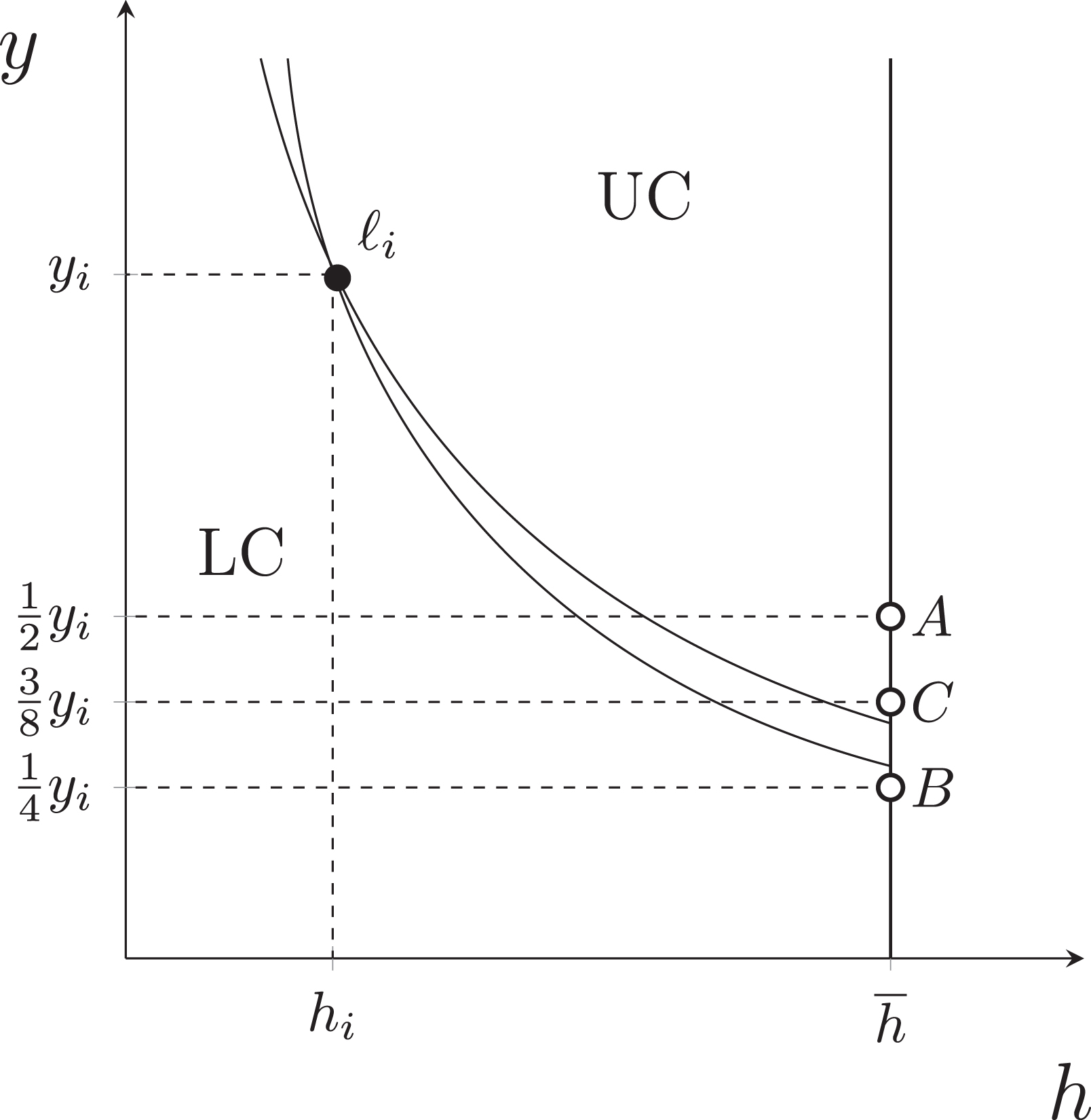
Illustration of the ABDC method
Illustration of the ABDC method
There are several novelties in this method compared to standard contingent valuation methods. First, the ABDC method captures more detail about individuals’ indifference curves by fixing the level of one dimension in the hypothetical life situation and varying the other. This approach allows for a more flexible analysis of preferences using nonparametric techniques from demand analysis (Varian, 1982), enabling tests of specific aspects such as monotonicity and the validity of commonly used functional forms, while relaxing assumptions about completeness. Second, the ABDC method employs a bisectional algorithm to progressively narrow the bounds around the indifference set. After each choice, the algorithm halves the level of one dimension in the hypothetical life, keeping the other fixed, which increases the precision of the estimates. Third, the ABDC method allows individuals to indicate that they cannot compare two alternatives by selecting an “I don’t know” option. This option may enhance the validity of estimates compared to methods that force respondents to make a choice, which may lead to phenomena as “yes-saying” or other heuristics. Offering the “I don’t know” option aligns furthermore with behavioral versions of equivalent income that relax the assumption of completeness. (see Fleurbaey and Schokkaert, 2013).
Table 2 provides an overview of some advantages and disadvantages of the ABDC method. As an extension of the bidding game elicitation mechanism, the ABDC method is potentially subject to starting-point biases that could influence the elicitation of equivalent income. Evidence from the contingent valuation literature suggests that this may impact both the point estimates and uncertainty intervals derived. For example, Dubourg and Loomes (1997) find that the starting bid influenced the best estimate of the respondents’ WTP, as well as uncertainty intervals in an iterated bidding game experiment similar to the ABDC. Additionally, eliciting preferences across more than two dimensions (i.e., constructing an indifference surface) is complicated by the large number of dichotomous choices required, which can lead to respondent fatigue and is likely less efficient than multi-attribute valuation methods (e.g., choice experiments) that are discussed in the next section. Nevertheless, the ABDC method may be valuable for researchers interested in measuring equivalent income directly rather than the trade-offs between the different well-being dimensions. For example, one can elicit the WTP for attaining the reference levels across multiple dimensions at once.
| Example | Advantages | Disadvantages |
|---|---|---|
| • Imagine two possible lives: your own and another . Which life would you choose? | • Elicitation of various points along the indifference curve, not just WTP. • Cognitively easier for respondents than open-ended questions. • Aligns with behavioral economic interpretations of the equivalent income. |
• Staring-point bias, preferences may be influenced by starting values. • WTP values are provided on an interval. • Many questions may be required to elicit indifference surfaces in multiple dimensions. |
By combining data generated by the ABDC method with standard assumptions about preference relations, such as transitivity, monotonicity, and convexity, the method can be employed to map individual indifference sets in a nonparametric manner. In their study, based on an online survey of 2,575 respondents from the United States, Decancq and Nys (2021) provide bounds on indifference sets through the individual’s actual life situation. Alternatively, data from the ABDC method can also be employed to test these preference assumptions and to assess consistency with commonly used functional forms in the literature. Decancq and Nys (2021) find that 17.5% of respondents make choices that violate monotonicity and transitivity, while approximately 9.5% fail tests of transitivity and convexity. About one third of respondents display choices inconsistent with a constant elasticity of substitution between income and health; inconsistency rates are higher for linear (95.4%), Cobb-Douglas (71.8%), Leontief (48.7%), and kinked linear (70%) preferences. Burone and Decancq (2023) apply the ABDC method to a representative sample of 2,048 individuals in the Netherlands to measure equivalent incomes in the three-dimensional income-health-social interactions space directly, without mapping the full indifference surface. Their study also allows for a comparison between the ABDC method and other approaches, results to which we will return in section 7.
Multiattribute methods
Data from multiattribute methods
The design and implementation of the multiattribute methods involves several stages. First, researchers must select the relevant attributes and corresponding levels for the good being valued. This selection process typically draws on theoretical insights and pretesting to ensure that the attributes and levels are realistic. In the context of equivalent incomes, these attributes correspond to relevant life dimensions. Next, researchers construct a set of alternatives from these attributes and levels, aiming for precise and efficient estimation of each attribute’s relative contribution. This often requires an experimental design that is orthogonal (i.e., uncorrelated attribute levels) and balanced (i.e., each attribute level appears an equal number of times across the experiment). Such designs can be created using orthogonal arrays or statistical software. Following this, alternatives are grouped into choice sets using various methods (see Johnson et al., 2013) or presented directly. Finally, the survey is conducted to elicit individuals’ preferences for the different attributes.
There are two broad categories of multiattribute methods: choice experiments and conjoint analysis. Choice experiments can be subdivided into two main forms. The first, discrete choice experiments, present individuals with sets of two or more alternatives, one of which is often a status quo option. In these experiments, respondents are typically asked to make a series of choices between the presented alternatives, allowing researchers to capture detailed information on their preferences. The second form, rank-order choice experiments, requires respondents to rank the presented alternatives according to their (ordinal) preference relation.
Conjoint analysis, by contrast, incorporates cardinal aspects of preference intensity. One popular approach in this category is the contingent rating method, where respondents rate hypothetical scenarios on a semantic or numerical scale (usually from 1 to 10) based on their preferences. Another approach, pairwise comparisons, is similar to discrete choice experiments in presenting two alternatives, but it asks individuals to rate the strength of their preference for one alternative over the other (e.g., “somewhat prefer” or “strongly prefer”) on a scale. This approach thus combines elements of discrete choice experiments and contingent rating, capturing both choice and the intensity of preference.
Estimation of preferences
Data from choice experiments and conjoint analysis are typically analyzed with parametric methods. Yet, the two categories rely on different theoretical frameworks. Decisions in a choice experiment are mostly modelled using random utility theory, which assumes that respondents’ preferences can be represented by a specific parametric functional form based on observable attributes of an alternative plus a random error component, capturing unobservable factors that influence choice (McFadden et al., 1973). This approach is related to the method described in section 4.2, with the main difference being that two alternatives are compared in choice experiments, whereas a reported WTP is compared with a deterministic benchmark in the earlier method. Different assumptions regarding the distribution of random error terms in a random utility model yield different discrete choice models. For instance, assuming normally distributed errors leads to a multinomial probit model, while assuming errors follow an extreme value distribution results in the conditional (or rank-order) logit model. The parameters of these models are estimated from observed choices or rankings using maximum likelihood and can provide WTP estimates if a monetary attribute (e.g., income or cost) is included.
We illustrate how preferences can be estimated with a basic discrete choice model. Suppose individuals are presented with choices between two or more hypothetical life situations, as has been used in previous empirical studies. Under the assumptions of random utility theory, the probability of individual choosing a hypothetical life is given by:
where is a function that specifies how an individual’s utility depends on observable factors and captures a set of random unobservable factors that influence choice but are not included within . These unobservable factors are particularly salient in stated preference studies as individuals may vary in the attention they give to the choice task or in how they account for unlisted attributes (Train and Weeks, 2005). The welfare interpretation of the model depends on whether represents optimization errors or idiosyncratic preference factors. Assuming an extreme value distribution of these unobservable factors leads to the logit case, in which a closed form for the choice probability is obtained:
Further assuming that is linear, we have:
where is the income level of a hypothetical life and includes all other nonmonetary aspects of the described life, such as health and social interactions. The coefficients of equation (4) can be estimated via maximum likelihood. Marginal rates of substitution can be computed by taking the ratio of these coefficients.
Preference heterogeneity can be introduced via interaction terms or by specifying more complex models. Advances in simulation methods enable researchers to estimate both the distribution of preferences within a population and individuals’ positions within this distribution, based on their sequence of choices, using mixed logit models (see McFadden and Train, 2000; Train, 2009). However, these models require the researcher to specify the shape of the preference distribution from the outset, the parameters of which are estimated from respondents’ choices. The problem is that this distribution is unknown and assumptions regarding it are likely to be arbitrary.
Unlike choice experiments, where respondents are asked to rank life situations and express ordinal preferences, conjoint analyses elicit the intensity of preference. WTP values can be estimated from contingent rating or pairwise comparison data in various ways. In the contingent rating method, one can estimate a linear preference function and take the ratio of the dimension coefficients to estimate marginal rates of substitution (Roe et al., 1996). Pairwise comparison data can be analyzed similarly, with the right-hand side of the model containing differences between the dimensions across alternatives rather than levels (see Magat et al., 1988). Hanley et al. (2001) notes that many pairwise comparison studies respecify the ratings as ordinal variables indicating choice, allowing analysis within a random utility theory framework, although this discards the additional preference intensity information. Nevertheless, this information can be incorporated as follows.
Assume that individual indicates their strength of preference on a cardinal scale from 0 to 10 between a pair of hypothetical life situations . The lower and upper bounds of this scale reflect a strong preference for either one of the hypothetical life situations. Denote the differences in the income and nonmonetary dimensions across pairs of life situations as and respectively. The researcher estimates the following equation using ordinary least squares:
where the ratio of two coefficients () is equal to the respondent’s marginal rate of substitution between income and the nonmonetary dimension. The model is flexible enough to capture group-level preference heterogeneity by introducing interaction terms between the coefficient and sociodemographic variables. The pairs of life situations could also be varied using an algorithm to calculate individual-level marginal rates of substitution (see Magat et al., 1988).
Advantages and disadvantages of multiattribute methods
Choice experiments have been argued to have several advantages over other preference elicitation methods (see Hanley et al., 2001). First, they provide a theoretically grounded framework with which to identify trade-offs between different attributes of nonmarket goods. While contingent valuation methods can also be used to estimate the value of different attributes (i.e., through a series of valuation questions), the process is usually more costly, cumbersome, and inefficient. Second, the outputs of choice experiments are more generalizable to other scenarios, given that the method focuses on valuing attributes rather than the nonmarket good as a whole. For instance, the estimated coefficients can be used to predict choices across other alternatives with similar attributes. Third, they provide opportunities for learning and preference discovery via repeated choices. Discrete choice models are flexible enough to account for this process (e.g., mistakes during preference formation) through the inclusion of the random utility term (Lancsar and Louviere, 2006). Lastly, choice experiments avoid the use of explicit money valuations, which may be subject to phenomena such as protest votes, as described in the case of contingent valuation methods in the previous section.
Nevertheless, choice experiments face several limitations:
-
Cognitively demanding: The overall precision of choice experiment estimates depends not only on the statistical efficiency of the underlying experimental design but also on the response efficiency, i.e., the degree of measurement error resulting from respondents’ mistakes or nonoptimal choice behavior (Johnson et al., 2013). Choice experiments can be cognitively demanding for respondents to answer if they have to consider many different attributes or alternatives simultaneously when making a choice. They may also have to make these choices a number of times. The overall complexity of the choice experiment may therefore lead to respondent fatigue or the use of heuristics, i.e., simplifying strategies that are not in line with the principle of utility maximising behavior. Such effects may contribute to the error term of the model (i.e., lower response efficiency), thereby reducing the precision of the parameter estimates. On the other hand, making choices seems to be more natural and less cognitively demanding than looking for indifference between two situations (as is often required for contingent valuation applications). For instance, Attema and Brouwer (2013) find that choice tasks yield more internally consistent responses than matching (i.e., searching for indifference) tasks.
-
Nonattendance bias: A key underlying assumption in a choice experiment is that respondents consider all the attributes of each alternative when making a choice or ranking. In practice, however, choice experiments may be susceptible to nonattendance bias, whereby respondents make their choices based on a subset of the attributes presented. There are several possible reasons why this might occur. Respondents might use simplifying strategies to make choices if the number of alternatives or attributes is too large to process. Alternatively, respondents may consider only one attribute of the alternatives to be important, leading to lexicographic orderings. Several methods have been proposed to correct for this bias. Hole (2011), for instance, proposes an endogenous attribute attendance model that adjusts the standard conditional logit formula for nonattendance bias (based on a set of observable respondent characteristics). These corrections are tricky, however, as it is difficult to distinguish between nonattendance bias and genuine lexicographic preferences.
-
Restrictive preference assumptions: The estimation methods are parametric and therefore impose some structure on individual preferences over observable attributes. Several challenges are relevant in this regard. First, there may be complex interactions between attributes that cannot be adequately modelled using standard choice models. Second, there may be attributes that are omitted from the experiment but are important determinants of choice. Respondents may also infer changes in these omitted attributes from the presented alternatives, which could lead to bias in the parameter estimates and reduce precision. In addition, these challenges make it difficult for researchers to measure the total value of a change in the provision of a nonmarket good. This is because choice models often assume that the value of an alternative is equal to the sum of its parts, i.e., the observed attributes (Atkinson and Mourato, 2015). Hanley et al. (2001) argue that this additive framework may be problematic as certain attributes may be missing and respondents may not value “whole” goods in this way. They point to evidence from several studies indicating that discrete choice experiments provides larger estimates of total value than contingent valuation. Such concerns are particularly relevant for the measurement of well-being using the equivalent income.
-
Preference heterogeneity: Unlike contingent valuation methods, choice experiments are unable to provide direct measures of WTP at the individual level. In standard conditional logit models, preference heterogeneity can be captured at the grouplevel via interaction terms. Mixed logit models offer more flexibility in the modeling of preference heterogeneity but only provide estimates of individual parameters based on strong parametric assumptions about the functional form of individual preferences as well as how these preferences are distributed across the population.
We summarize some advantages and disadvantages of specific multiattribute methods in Table 3. The key advantage of choice experiments (in row 1 and 2) over conjoint analysis (in row 3 and 4) is that they provide estimates of WTP that are consistent with random utility theory. Meanwhile, conjoint analysis methods can provide more information, i.e., intensity of preference, than standard choice or ranking tasks. However, they also rely on relatively strong assumptions about inter- and intrapersonal scale use. It is perhaps for this reason that conjoint analysis has failed to garner popularity with economists (Hanley et al., 2001).
| Method | Example | Advantages | Disadvantages |
|---|---|---|---|
| Discrete choice experiment | • Which life would you prefer? Please choose from the two options below. | • Mimics real-life decision-making processes. • Linked to RUT, welfare consistent estimates. • Useful for predicting choices or impacts of policy. |
• Respondents might find it difficult to make multiple choices in succession. • Only indicates ranking not strength of preference. |
| Rank-order choice experiment | • Please rank the following life situations according to your preference. | • Provides relative preference information, not just choice. • Linked to RUT, can provide welfare consistent estimates. • Useful for small samples as provides more information per respondent. |
• May be cognitively difficult to rank many alternatives at once. • Only indicates ranking not strength of preference • Requires more complex design and modelling techniques (e.g., rank-order logit). |
| Contingent rating | • On a scale of 0-10, please rate the following hypothetical life situations. | • Allows respondents to express their strength of preference. • Analysis relies on simple statistical techniques, e.g., OLS. |
• Relies on strong assumptions of cardinal and interpersonally comparable scale use. • Cognitively challenging to rate alternatives |
| Pairwise comparisons | • Which life would you prefer? Please indicate your strength of preference below. | • Reduces cognitive load by allowing respondents to rate two alternatives at a time. • Ratings can also be analyzed as implied choices. |
• Rating multiple pairs imposes larger cognitive load than discrete choice experiments |
Reliability and validity of multiattribute methods
In contrast to contingent valuation, evidence on the reliability and validity of discrete choice experiments remains relatively limited and mixed. Haghani et al. (2021) provide a review of criterion and convergent validity in discrete choice experiments by examining hypothetical bias across four fields: consumer, environmental, health, and transport economics. Their review covers 57 peer-reviewed studies, more than half of which report significant hypothetical bias. The authors identify two key issues complicating hypothetical bias testing across studies. First, a true benchmark preference is often missing, making it challenging to assess hypothetical bias. Second, hypothetical bias likely varies with the choice context. Notably, the field of health economics reflects a different perspective on the extent of this bias compared to other fields, likely due to differences in perceived importance. For example, health-related surveys may prompt respondents to take choice tasks more seriously than questions about consumer goods, such as foods or beverages. Conversely, protest responses seem more frequent in health contexts. Additionally, health-focused choice experiments often examine private goods, while environmental surveys tend to concern public goods, which may be more vulnerable to other biases (e.g., warm glow and free-rider effects).
In their systematic review of 107 studies within environmental economics, Rakotonarivo et al. (2016) assess the reliability and validity of choice experiments. For reliability, they examine studies that incorporate test-retest trials (repeating the same survey at different times), as well as variations in framing, the provision of additional deliberation or information, and experimental design changes (including adjustments to attributes, levels, and design parameters). Nearly half of the estimates (45%) showed sensitivity to minor design changes. Regarding validity, the authors evaluate studies testing for criterion ( =11), convergent ( =13), and construct validity ( =30), with construct validity assessments including conformity with standard rational choice axioms and attribute non-attendance. The results are mixed at best: no criterion validity evidence was found, and only limited convergent validity with other methods. While most respondents passed monotonicity tests, high levels of self-reported attribute nonattendance were reported. Additionally, only two of six studies testing for scope effects found evidence supporting these effects.
There are various other studies testing the convergent validity of choice experiments within the field of health economics. For instance, several studies find that the WTP values elicited from discrete choice experiments are much higher than those obtained from contingent valuation (Ryan et al., 2004; van der Pol et al., 2008; Ryan and Watson, 2009; Bijlenga et al., 2011; Danyliv et al., 2012). Danyliv et al. (2012) review this literature in more detail and highlight potential causes of this difference, including restrictive assumptions regarding the linearity of the utility function (as discussed earlier), the absence of substitutes (e.g., opt-out alternatives), and specific aspects of the experimental design (e.g., the range of the price attribute). Comparisons between other forms of choice experiment and contingent valuation are less common in health economics. A rare example is provided by Magat et al. (1988), who find that morbidity valuations obtained from the pairwise comparison and contingent valuation methods differ considerably, with the former yielding higher WTP estimates.
These findings also connect to evidence on preference reversals observed between matching and choice tasks within the behavioral economics literature (Tversky et al., 1988; Lichtenstein and Slovic, 2006b). In a matching task, respondents adjust a single dimension of an alternative to achieve equivalence between two alternatives, similar to contingent valuation when a monetary attribute is adjusted. In a choice task, respondents’ preferences are inferred from their choices between two alternatives, one of which is iteratively varied until a point of indifference is reached. Tversky et al. (1988) argue that the discrepancy between preferences obtained from these two methods can be explained by the prominence effect, whereby respondents focus more on the most important (or prominent) attribute when making choices rather than matching. Attema and Brouwer (2013) demonstrate that this effect is also prevalent when eliciting preferences over health states and life span, in the form of QALYs. Pinto-Prades et al. (2018) find that the prominence effect may be mitigated to some extent by using nontransparent methods that hide the underlying objective of an iterated choice task. Such findings may also affect the elicitation of equivalent income using variations of these methods: open-ended/payment cards in the case of matching and ABDC (see section 4.6) in the case of choices.
Multiattribute methods and the estimation of equivalent income
In multiattribute approaches, the good to be valued is viewed as a function of various attributes. In the context of estimating equivalent incomes, the good to be valued is a life situation that can be described using several life dimensions. While multiattribute methods have not yet been used in the literature to estimate equivalent incomes, the relevant preferences can be estimated based on comparisons or valuations of descriptions of hypothetical life situations, sometimes referred to as vignettes.
When relying on a choice experiment, respondents are asked to compare several life situations of which the attribute level in the life dimensions are experimentally varied. Recall that the actual life situation of individual is denoted by and the reference life situation . Using the estimated preference parameters from the linear model in equation (4), for instance, the actual and the reference life situation are equivalent if:
where represents, as before, the reference level of the nonmonetary dimensions and the equivalent income. By rearranging this equality, we can easily obtain an expression for the equivalent income:
Preference heterogeneity can be accommodated by including interaction terms with sociodemographic variables in the specification of in equation (4). We will return to this procedure when describing the life satisfaction method in section 6.2.
When using the contingent rating (or factorial survey) method, respondents rate several vignettes, i.e., hypothetical life situations described across various life dimensions. These ratings allow the straightforward estimation of (group-level) preferences.Van Loon and Decancq (2022), for instance, present each respondent with seven vignettes, each describing a hypothetical life situation across six dimensions. The respondents, 800 older adults, are given an 11-point satisfaction scale for their response.
“Please read the following life description carefully.
You have [moderately severe] physical or mental health problems.
You have [several times per week] contact with family or friends.
The total net household income is [€5,000.00].
You do [once per week] a hobby or leisure activity.
You do [several times per week] a useful or meaningful activity.
You spend [less than once per week] time on religion or spirituality.
How satisfied would you be if you were in this situation?”
The bracketed words indicate levels that varied experimentally across vignettes. Van Loon and Decancq (2022) employ a multilevel model to estimate preferences based on the ratings of the vignettes, incorporating error terms at both the vignette and respondent levels. Although the authors do not compute equivalent incomes, this could be done with the estimated parameters using equation 6. A total of 154 respondents rated vignettes across five waves, from May to December 2020, enabling a test of the temporal reliability of the estimated preferences. In 6 of 10 cases, the hypothesis of parameter stability could not be rejected.
Life satisfaction method
Self-reported well-being data
A relatively recent literature explores the potential of using self-reported well-being measures (SWB) to inform policymaking decisions. An example is the life satisfaction question from the European Social Survey:
“All things considered, how satisfied are you with your life as a whole nowadays? Please answer using this card, where 0 means extremely dissatisfied and 10 means extremely satisfied.”
Data on SWB have by now been collected for thousands of respondents throughout the world with large-scale surveys. The literature analyzing this data has followed two distinct paths. One path interprets the responses as cardinal measures of utility (e.g., Layard et al., 2008), while the other seeks to recover information about ordinal preferences from the responses (as in the previously discussed contingent rating method). These preferences can then be used to value nonmarket goods (e.g., Clark and Oswald, 2002; Ferrer-i-Carbonell and Van Praag, 2002) or to construct measures of well-being (e.g., Decancq et al., 2015a). Typically, researchers regress life satisfaction scores on income and nonmonetary dimensions of well-being, controlling for other personal characteristics of the respondents. The estimated coefficients can then be used to derive the marginal rate of substitution between income and a selected life dimension.
From a theoretical perspective, responses to the life satisfaction question capture experienced rather than decision utility. The former reflects an ex post evaluation of one’s situation, that is, after experiencing the consequences of different choices. In contrast, decision utility is based on choices made ex ante and reflects individuals’ beliefs about their consequences. We have already seen that choices can only be considered reliable indicators of well-being if they are made under ideal conditions, characterized by full information, correct beliefs, and an absence of behavioral distortions, among other factors (Hausman, 2011; Bernheim, 2016). Given that these conditions are rarely met in practice, some have argued that experienced utility (equivalently, SWB measures) may serve as a better indicator of informed preferences and, therefore, well-being (Decancq et al., 2015b).
From life satisfaction scores to equivalent income
To illustrate the estimation of preferences using the life satisfaction method, assume the existence of a satisfaction function that maps a life situation into a self-reported life satisfaction score, typically measured on a scale from 0 to 10. While this life satisfaction score is a cardinal value, it may also be informative about the underlying ordinal preferences, provided a consistency assumption holds (Decancq et al., 2015a).
Consistency assumption: if and only if for each individual .
Under this assumption, the marginal rates of substitution between dimensions can be estimated using a life satisfaction regression. The functional form of this regression can be flexibly chosen, but a common specification is a log-linear one:
where is the life satisfaction score given by individual in period , is their income (in logarithm), is a vector of nonmonetary life dimensions, and capture individual fixed effects and time effects, respectively, and is a set of sociodemographic control variables that capture how individuals use the reporting scales. The marginal rates of substitution depend on the coefficients and . Differences in scale use are captured by the fixed effects , time-varying control variables , and idiosyncratic error terms . These scaling differences reflect variations in ambitions and adaptation (Sen, 1985), or cultural differences in scale use (Johnson et al., 2005), and should not influence the equivalent income. Equivalent incomes are based solely on marginal rates of substitution, not on the specific cardinalization of the preferences. Indeed, equivalent income can be calculated, starting from the equivalence between the actual and the reference life situation:
Solving this equation for yields:
The value of the equivalent income depends on the actual income and the WTP, which depend on the estimated coefficients and and the difference between the actual nonmonetary dimensions and the reference values . It does not depend on any of the scaling variables.
More flexible forms (e.g., using Box-Cox transformations) of the model in equation (7) can be adopted to account for nonlinearities (see, e.g., Decancq and Schokkaert, 2016; Decancq et al., 2019). Group-level preference heterogeneity can be introduced by including interaction terms between the dimensions of life and sociodemographic variables indicating group membership in equation (7) (see, e.g., Decancq et al., 2015a; Decancq and Schokkaert, 2016). Because it is based on interactions in a regression analysis, the life satisfaction method can capture group-level preference heterogeneity, but not individual-level heterogeneity.
Advantages and disadvantages of the life satisfaction method
An important advantage of the method is that life satisfaction data are relatively inexpensive and easy to collect, as only one additional survey question is required. Major life satisfaction surveys (e.g., Gallup) target a representative sample in each country, allowing researchers to capture the preferences of the entire population. Although results from these large surveys may be affected by low response rates (Heffetz and Rabin, 2013; Benjamin et al., 2023a), such large samples are often unavailable for other methods that require more resources per respondent (e.g., choice experiments). Additionally, the method may be less susceptible to biases inherent to other stated preference methods (e.g., ordering and framing effects) as well as protest responses.
The life satisfaction approach, however, also has some disadvantages. Most importantly, the consistency assumption that underpins the method is empirically untestable. Researchers must therefore take this assumption as given when inferring preferences from predicted life satisfaction scores. There is a literature comparing hypothetical choices and hypothetical estimates of well-being (Benjamin et al., 2012, 2014b), which is providing indirect evidence. A key issue is that people may not maximize their own satisfaction with life but take account of their relatives in their choices, whether real or hypothetical. This means that choices and self-centred preferences may not be completely aligned, and therefore, consistency between life satisfaction and preferences cannot be directly assessed through the relation between life satisfaction and decisions.
The preference information derived with the life satisfaction method ultimately depends on the factors an individual considers when responding to a life satisfaction question and how those factors are weighted. It remains unclear which utility concept respondents apply in formulating their responses (Benjamin et al., 2023a).
Furthermore, there is an ongoing debate on whether self-reported well-being scores should be interpreted as a measure of an individual’s happiness (in which case they could be considered an important life dimension and thus a component of the preferences; see Benjamin et al., 2012; Adler et al., 2017) or as a reflection of underlying preferences (Decancq et al., 2015a). Fleurbaey and Schwandt (2016) provide evidence supporting the latter view.
In addition, there are several econometric challenges posed by the estimation of the life satisfaction regression in equation (7). Perhaps the two most important are:
-
Endogenous regressors and measurement errors: More satisfied individuals may earn higher incomes. Prior studies have shown that controlling for this type of bias via instrumental variables increases the income coefficient considerably (Knight et al., 2009; Powdthavee, 2010; Himmler et al., 2021), leading to lower WTP estimates for the nonmonetary dimensions and, thus, higher equivalent incomes. On the other hand, it has also been argued that income is measured with considerable error, which could bias its effect toward zero, bias the WTP estimates for the nonmonetary life dimensions upward and the estimates of equivalent income downward (Himmler et al., 2021).
-
Scaling effects: An implicit assumption of equation (7) is that, conditional on the included scaling variables, all individuals use the reporting scale in the same way when rating their life satisfaction. Bond and Lang (2019) refer to this as the assumption of a common reporting function, which they consider to be “unlikely to be correct” (see also Kaiser and Oswald, 2022). Indeed, scale use may depend on various observable (such as the life dimensions themselves) and unobservable factors, the latter of which are problematic if correlated with the variables of interest. One approach to address this bias involves using vignettes that describe hypothetical life situations to anchor the scale on which people report their life satisfactions (King et al., 2004). Yet, the use of anchoring vignettes requires that individuals rate the vignettes on the same scale as they evaluate their own life satisfaction (“response consistency”) and that each individual rates the vignettes in the same way (“vignette equivalence”). When preferences are heterogeneous, the latter assumption is strong (see Benjamin et al., 2023b for a recent discussion).
Reliability and validity of the life satisfaction method
We are unaware of any systematic analyses assessing the validity of marginal rates of substitution derived from the life satisfaction method. Some studies, however, have evaluated convergent validity by comparing WTP estimates obtained from the life satisfaction method with those derived from other methods:
-
Dolan and Metcalfe (2008) compare WTP estimates from contingent valuation and the life satisfaction methods within an urban regeneration project in the UK. They find that estimates derived from the life satisfaction method are substantially larger than those obtained via contingent valuation.
-
Benjamin et al. (2014b) survey medical students, comparing their choices of residence with anticipated levels of self-reported well-being in each scenario. They estimate marginal rates of substitution across residence dimensions using both data sources and find substantial differences between the two sets of estimates. This result holds across different measures of self-reported well-being, such as happiness and life satisfaction, and the authors note that these findings relate to anticipated, not experienced, subjective well-being.
-
Murtin et al. (2017) estimate the WTP for life expectancy gains across OECD countries. Their life satisfaction-based method, using individual-level data, produces WTP values far exceeding those from the value of statistical life literature. They suggest that individual-level measurement error may be influencing these results. When re-estimating the model with country-level data, their results align more closely with values reported in the literature.
-
Akay et al. (2020, 2023) estimate indifference maps over income and leisure time using both the life satisfaction method and labor supply choices (i.e., revealed preferences). Constructing money-metric utilities with both methods, they find a high degree of correlation between welfare rankings derived from the two approaches, though some discrepancies persist.
-
Humphreys et al. (2020) compare WTP estimates for Olympic gold medals derived from the life satisfaction and contingent valuation (referendum) methods. They report that the life satisfaction-based estimates significantly exceed those obtained via contingent valuation.
Regarding construct validity, the consistency assumption remains problematic since it cannot be empirically tested. Thus, we cannot verify whether individuals’ life satisfaction scores correspond with their underlying ordinal rankings of life situations. This links to a broader issue of whether life satisfaction scores reflect any standard economic notion of utility. Benjamin et al. (2023c) present evidence on this front using an online survey that probes respondents on how they interpret and answer different self-reported well-being questions. Their findings suggest that respondents’ answers do not clearly correspond to notions such as lifetime, forward-looking, or period utility, nor do they align with self-centred utility. Instead, many respondents incorporate other-regarding preferences, including considerations for family members. However, their research indicates that minor adjustments in the wording of self-reported well-being questions may improve alignment with specific utility concepts.
Comparison of methods
We now turn to the second set of evaluation criteria, focusing on the scope of each method in relation to the researcher’s theoretical objectives (measuring equivalent incomes, estimating marginal rates of substitution, or mapping indifference curves) and the desired degree of preference heterogeneity (at the individual or group level).
Table 4 summarizes the comparison of the methods. In the second column of the table, “easier for” signifies that a method is readily applicable to estimating a particular concept. Yet, this does not imply that current estimation methods have satisfactory statistical power or that further data analysis is unwarranted. For instance, life satisfaction regressions are straightforward to implement using standard survey data with a life satisfaction question, though, as discussed in the previous section, they also have significant limitations.
| Theoretical objectives easier for estimating… | Preference heterogeneity at the level of… | |
|---|---|---|
| Contingent valuation | ||
| Open-ended | equivalent income | Individual |
| Referendum | equivalent income | Group |
| Payment cards | equivalent income | Individual |
| Bidding game | equivalent income | Individual |
| ABDC | equivalent income, indif. sets | Individual |
| Multiattribute methods | ||
| Discrete choice | MRS, indif. curves | Group |
| Ranking | MRS, indif. curves | Group |
| Contingent rating | MRS, indif. curves | Group |
| Pairwise comparisons | MRS, indif. curves | Group |
| Life satisfaction method | equivalent income, MRS, indif. curves | Group |
The third column of the table addresses the degree of preference heterogeneity. Generally, nonparametric approaches allow for analysis at the individual level, whereas parametric methods require data pooling and are typically limited to the group level. An individual-level analysis is in line with the principle of individual sovereignty, a cornerstone of the equivalent income approach, and a nonparametric approach avoids potential functional misspecifications. In fact, group-level estimates may not accurately represent the preferences of any actual individual within the target population. Concrete policy analysis, however, often requires the measurement of well-being in counterfactual scenarios—an objective that is difficult to achieve without a parametrized model. Furthermore, parametric models that incorporate a stochastic error component can explicitly account for measurement errors or respondent mistakes in the preference elicitation process. Some advancements in choice experiments also enable the estimation of preference distributions or approximate individual preferences, provided that parametric assumptions about the distribution of preference parameters are specified a priori (Train, 2009).
We begin with contingent valuation methods. Apart from the referendum approach, contingent valuation methods permit the highest degree of preference heterogeneity, enabling WTP estimates at the individual level. This allows researchers to construct well-being measures, such as equivalent income, efficiently by prompting respondents for an overall valuation, sometimes with a single question. However, the elicitation of marginal rates of substitution and indifference curves using these methods is less straightforward, as it necessitates parametric functional form assumptions and typically limits preference heterogeneity to the group level. The ABDC method offers greater promise in this respect, though it requires multiple questions to approximate indifference curves accurately. For example, Decancq and Nys (2021) required respondents to make 10 choices to approximate an indifference set in a two-dimensional space. In particular when the number of dimensions increases, researchers are likely to encounter the so-called curse of dimensionality.
Multiattribute methods and the life satisfaction approach, on the other hand, are more efficient for eliciting marginal rates of substitution between multiple dimensions of well-being and for mapping indifference curves. This efficiency is due to their reliance on experimental designs and parametric estimation techniques. Multiattribute methods are less efficient for estimating well-being levels directly, as respondents must make multiple choices to reveal the relative importance of each dimension. As the number of dimensions increases, the required choices per individual or across the sample also rise. By contrast, contingent valuation and life satisfaction methods require only a single question. Multiattribute methods can, however, focus on eliciting WTP or WTA for a set of simultaneous attribute changes, making them comparable to contingent valuation methods, particularly the bidding game.
The table discusses the case in which well-being is measured by equivalent income. When other notions of well-being are applied, important adjustments to its contents may be necessary. For instance, if VNM (von Neumann-Morgenstern) utility, suitably normalized, is the chosen well-being measure, then the table remains valid, though there are questions concerning whether life satisfaction methods can accurately measure VNM utility. It is sometimes assumed in the literature (e.g., Finkelstein et al., 2013) that life satisfaction scores can be directly interpreted as measures of VNM utility. However, this assumption is debatable; it seems more reasonable to regard life satisfaction scores, which are based primarily on experienced utility, as reflecting final outcomes rather than capturing risk attitudes (see also Oswald, 2008). The table would appear very different if self-reported well-being, identified with life satisfaction, were used as the well-being measure. In that case, all methods except life satisfaction would be unsuitable for estimating well-being, while life satisfaction scores would provide direct well-being estimates at the individual, not merely group, level.
More detailed assessments of the various methods are summarized in Tables 1, 2, and 3, particularly in terms of cognitive load, potential biases, nonresponses, protest answers, and the elicitation of intervals versus point values. Clearly, no single method excels across all relevant criteria, and section 9 aims to draw lessons from this review. Additionally, certain aspects of different methods can be combined, such as appending an open-ended question following a payment card elicitation to obtain a point estimate of WTP.
Empirical evidence on the estimation of equivalent incomes
In this section, we review the emerging empirical literature that applies the preference elicitation methods discussed previously to compute equivalent incomes and other preference-based measures of well-being. The early literature, which sought to compare living standards across countries, primarily relied on revealed preference data to estimate average preferences for valuing dimensions such as longevity and leisure time (Fleurbaey and Gaulier, 2009; Jones and Klenow, 2016). Here, we focus on stated preference studies that elicit equivalent income at a more granular level. We begin with research employing contingent valuation methods, then turn to studies using multiattribute approaches, and conclude with work based on the life satisfaction method.
Contingent valuation
Empirical studies using the contingent valuation method to elicit preferences have primarily focused on life situations defined in the income (or consumption) and health domain.
Fleurbaey et al. (2013) elicit WTP values for perfect health using a payment card format. They ask individuals to state the absolute decrease in personal consumption they would have accepted over the last year to be in perfect health (in addition to the health expenditures already incurred). Response cards range from “0 euros” to “more than 1500 euros” per month. Their pilot study was carried out with 542 respondents from the Marseille area, of which 20% either refused to answer the question or did not know how to answer. They distinguish between “severe” and “less severe” health problems and estimate indifference maps at the group level.
Building on this study, Schokkaert et al. (2013) and Samson et al. (2018) carry out a payment card contingent valuation study with 2,413 French respondents, with a focus on the valuation of health outcomes for individuals with hypertension. Self-assessed health is measured on a 0-100 scale and respondents are asked how much income they would be willing to give up to have been in perfect health over the past 12 months. The focus in Samson et al. (2018) is on the application of the equivalent income for priority setting in health insurance.
Abasolo et al. (2018) use a similar payment card method to elicit equivalent income with respect to health and relationship problems. Instead of using absolute amounts, the authors use cards with percentage decreases in consumption. Their online sample is relatively small with only 52 respondents. However, their qualitative debriefing questions yield important insights. For instance, some individuals were puzzled that consumption would go down after health has improved (i.e., they believed better health would allow them to increase their spending).
In their book, Capéau et al. (2020) analyze 1,857 respondents in the Measuring Equivalent Income (MEqIN) dataset, which includes contingent valuation questions regarding individuals’ WTP for health, housing, and ideal job characteristics. The question asks respondents how much they would be willing to reduce their monthly consumption over the next year to enjoy the reference level of the non-monetary dimension. The survey utilizes a payment card method with options ranging from “0 euros” to “more than 1500 euros”. The nonmonetary dimensions are presented to individuals on a scale ranging from 0 to 100.
Decancq and Nys (2021) apply the ABDC method in an online survey of 2,260 respondents in the United States. Because the framework allows for incomplete preferences, respondents can indicate that certain life situations are not comparable. The authors assess comparability across individuals by examining whether the extended upper contour set of the better-off respondent and the extended lower contour set of the worse-off respondent intersect. If these sets do not intersect, the pair can be ranked. Using this criterion, approximately one fifth of all respondent pairs can be ordered. In about half of the pairs, the intervals containing the equivalent incomes do not overlap, allowing for a robust comparison of their equivalent incomes.
Multiattribute methods
Published studies employing multiattribute methods to elicit preferences for computing equivalent income remain scarce. A notable exception is the recent work by Ta et al. (2024), who use an online survey of about 7,000 UK respondents to elicit preferences across seven well-being dimensions: physical and mental health, loneliness, income, employment, housing, and neighborhood safety. The authors further investigate preference heterogeneity by gender, age, and income and assess the temporal stability of preferences.
Nonetheless, a number of studies have applied multiattribute methods to assess the relative importance of different well-being dimensions, outside the equivalent income framework. We briefly review some examples later.
Adler and Dolan (2008) ask a small group of students in the US and UK to rank hypothetical life situations (which they call the “different lives” method) that differ in terms of income, life expectancy, health, and self-reported well-being. They find that respondents place greater weight on health and happiness than income and life expectancy.
Benjamin et al. (2012) present about 2,700 respondents in the US with pairs of “possible lives” that differ in many aspects, such as the amount of sleep one has due to a job and the level of income that job provides. They ask individuals to state which life would make them more satisfied and which one they would choose. Their results indicate a high degree of correlation between the responses to the two questions.
Benjamin et al. (2014a) ask 4,600 respondents to make pairwise comparisons of different aspects of well-being. They use a rating scale that asks individuals whether they “Much prefer,” “Somewhat prefer,” or “Slightly prefer” one of two options. They use OLS to analyze the relative marginal utilities associated with each aspect of well-being.
Adler et al. (2017) present large samples of respondents in the US and UK (total sample size of about 13,000 respondents) with choices between life situations described by income, health, family life, career goals, and knowledge. They also include measures of life satisfaction within the hypothetical life situations to see whether respondents prefer life situations with higher levels self-reported well-being. The results suggest that people often choose the life with higher levels of satisfaction and that health is also an important factor.
Watson et al. (2019) derive dimension weights for the Oxford Index of Multiple Deprivation using a discrete choice survey with a sample of 1,000 respondents in the UK. They ask respondents to compare hypothetical life situations with different levels of, e.g., income, employment, health, and housing quality and to state which life requires most support from the government. The results show that individuals place more weight on health, and housing quality relative to employment.
Fujiwara (2021) asks 282 respondents to compare the life situations of two hypothetical individuals and rate which would be more satisfied with their life situations. Following this, he prompts the respondent to record the level of satisfaction on a scale between 1 and 7. The study considers several dimensions: health, household income, unemployment, and ability to rely on family and friends.
Deyshappriya and Feeny (2021) use a variation of a standard discrete choice experiment, the so-called Potentially All Pairwise RanKings of all possible Alternatives (PAPRIKA) method to elicit the dimension weights of the Human Development Index in Sri Lanka. This method is an adaptive type of a discrete choice experiment that invokes the assumption of transitivity to identify and minimize the number of comparisons an individual is required to make. The weights from the method are derived using linear programming. McGillivray et al. (2023) use the same method to elicit weights in the UK.
Van Loon and Decancq (2022) ask 800 respondents to consider vignettes of possible life situations and rate their SWB in each. These vignettes describe various levels of different dimensions of life (health, income, social relations, leisure, engagement and religion) and are generated using a fractional factorial design. Once individuals have rated different vignettes, they estimate the relative weight of each dimension.
Life satisfaction method
A third strand of the literature has adopted the life satisfaction approach. Likely due to the widespread availability of life satisfaction data across countries, this strand has grown in recent years.
Decancq et al. (2015a) proposed the use of life satisfaction data to construct the equivalent income measure. They utilize the Russia Longitudinal Monitoring Survey (RLMS) from the period 1995-2003 to estimate trade-offs between income, health, housing, and wage arrears, using equation (7). They correct for unobservable heterogeneous scale use, by including individual fixed effects in their regressions. Their results indicate that social welfare depends on the chosen well-being measure, with various measures (e.g., income, life satisfaction, and equivalent income) all yielding different distributions of well-being. They also document some degree of preference heterogeneity among different sociodemographic groups.
Over the past decade, a series of studies have relied on the life satisfaction method to estimate preferences for well-being measurement. These studies often compare the correlations between preference-based measures and standard well-being indicators such as income or life satisfaction, or examine the individuals identified as worst-off under different well-being measures. Decancq and Neumann (2016), for instance, compare across different well-being measures (including equivalent incomes and von Neumann-Morgenstern utilities) using cross-sectional data from the 2010 German Socio-Economic Panel (GSOEP), focusing on three dimensions: income, health, and labor status. They find strong correlations among well-being measures aggregating the three dimensions, whether preference-based or not, and weak correlations of such measures with life satisfaction or income. Decancq and Schokkaert (2016) adopt the life satisfaction method using two waves of the European Social Survey to estimate equivalent incomes across several European countries, incorporating dimensions such as health, social interactions, unemployment status, and safety. Again, they find that the choice of well-being measure matters, with some countries showing large shifts in rankings once nonmonetary dimensions are incorporated into the equivalent income. Defloor et al. (2017) compare results across different notions of subjective well-being as explained variable in equation (7) (life satisfaction, happiness, and perceived life value) and show that achievements in the dimensions of well-being matter more for equivalent incomes than individual preference heterogeneity. Yang (2018) use the life satisfaction method to estimate preferences for the dimensions of the Human Development Index based on data from the British Household Panel Survey (BHPS). These estimated preferences are then used in a “preference index,” which resembles the equivalent income approach but employs a different method to label indifference curves and enable interpersonal well-being comparisons. Ledić and Rubil (2019) estimate equivalent incomes using data from the European Quality of Life Survey (EQLS) and decompose the difference in inequality between income and equivalent income into two components: one reflecting the correlation between income and nonincome dimensions (and between income and individual preferences) and another arising from individuals’ differing positions in the equivalent income and income distributions. Decancq et al. (2020) interpret the equivalent income measure of well-being through the lens of the capability approach and apply the life satisfaction method to estimate preferences using Colombian data. They compare the identification of the worst-off under the equivalent income approach with alternative approaches, such as the Colombian Multidimensional Poverty Index (MPI) and find substantial differences. Finally, Mori and Sakamoto (2024) compare equivalent incomes with three well-being measures (income, life satisfaction, and the MPI) from the perspective of human dignity. Using data from an Indian Slum Survey in Delhi, the study finds that the life satisfaction method yields relatively low valuations for education and health.
A few studies have used the life satisfaction method to estimate preferences and compute equivalent incomes for addressing policy questions. Jara and Schokkaert (2017) assess the effects of different policy scenarios on income, self-reported well-being and the equivalent income, using an (ex ante) microsimulation tool. Their results indicate that the ranking of different policies depends on the well-being measure used. Decancq et al. (2025) use the life satisfaction approach to study the (ex post) impact of the introduction of a noncontributory social pension program (Pension 65) in Peru, highlighting its varying effects on the three main ethnic groups: Mestizo, Quechua, and Aymara. As welfare criterion they check whether the program has lifted recipients to a higher indifference curve.
Applications of the life satisfaction method illustrate how the equivalent income concept can be extended to domain-specific measures of well-being or applied in specific contexts. Schokkaert et al. (2011) and Ledić and Rubil (2021) use the life satisfaction method to estimate so-called equivalent wages, a concept that is designed to capture heterogeneous working conditions and job quality, in similar fashion as equivalent income captures differences in quality of life. Decancq and Michiels (2017) apply the life satisfaction approach to measure the concept of successful aging and compare it with objective and subjective measures of successful aging.
Reconnecting with the early literature, some recent studies have compared living standards by constructing equivalent incomes that combine information from revealed preference studies with estimates from life satisfaction regressions. Murtin et al. (2017), for example, construct equivalent incomes incorporating life expectancy and unemployment; see also Veneri and Murtin (2019) and Boarini et al. (2022). Trade-offs for the former are recovered from revealed preference studies on the value of statistical life while preferences for the latter are estimated using the life satisfaction method. The resulting equivalent income measure is utilized to measure the welfare loss from the Great Recession. They find that welfare decreased by a much larger rate for equivalent incomes than GDP per capita.
Discussion
Challenges for equivalent income elicitation
Several theoretical challenges extend to empirical implementation:
-
Dimensions for inclusion: Respondents may not only make different trade-offs between life dimensions but may also hold varying views on which dimensions are essential to a good life. Comprehensively listing these dimensions is likely challenging. For instance, Benjamin et al. (2014a) identify over 100 aspects of well-being in the literature that they randomly assign to respondents. Benjamin et al. (2017) suggest that this number could be closer to 2,000 aspects. With so many dimensions, evaluation becomes cognitively demanding, requiring separability assumptions to aggregate detailed aspects into a smaller set of higher-level dimensions. However, if the dimensions become too abstract, they may lose relevance to respondents’ lived experiences, reducing evaluation salience. Additionally, respondents may implicitly consider changes in dimensions not included in the stated preference task, potentially increasing error term variance and introducing systematic bias into the estimated coefficients.
-
Measurement of nonmonetary dimensions: The equivalent income approach often requires quantitative measurement of nonmonetary dimensions such as health, social interactions, and environmental quality. Accurately conveying changes in these concepts in a way that avoids varied interpretations is challenging. For instance, individuals may interpret ambiguous terms such as “high,” “medium,” and “low” differently, which can add error variance and bias in estimated random utility models. Additionally, the use of indices or arbitrary scales may introduce scaling effects, as respondents may interpret these scales differently (see Benjamin et al., 2017). This issue is particularly evident when health is measured as “self-perceived health status.”
-
Interactions between nonmonetary dimensions: Interactions between dimensions can complicate the estimation of their individual contributions to well-being. For instance, Abasolo et al. (2018) report that respondents struggled with the concept of sacrificing income to attain optimal physical or mental health, as improved health might enable higher earnings or better job prospects. Respondents in their study also highlighted these interdependencies when ranking hypothetical life scenarios. Another example is the link between health and social interactions: a housebound individual may be unable to attain their ideal social situation, even if the scenario asks them to imagine otherwise. This suggests that respondents may have difficulty distinguishing between their opportunity sets and preferences.
-
Monetary trade-offs: Some respondents may reject the idea of trade-offs between income and nonmonetary dimensions of life, which can lead to a high incidence of protest responses in contingent valuation surveys. Evidence on this issue within equivalent income surveys is limited. However, Fleurbaey et al. (2013) found that 20% of their 435 respondents reported they would not accept a lower income, even if it meant avoiding health issues experienced in the past 12 months.
-
Selecting reference levels: Within the equivalent income approach, WTP values are elicited with respect to a reference level of each life dimension. Though this reference level is ultimately a normative choice, a practical challenge arises if the level should align with respondents’ conceptions of an “ideal” situation. This can be complex if individuals have varying views on what is the “ideal” level of a dimension. Figure 4 illustrates a scenario where an individual’s “ideal” level of social interactions () is lower than the reference level set by the researcher (). If the WTP is elicited for (i.e., ) through an open-ended contingent valuation question, the researcher may not capture the maximum WTP for social interactions, which is actually . This issue highlights challenges in defining reference levels and raises questions about the relevance of standard validity tests, such as scope sensitivity. Methods that capture more details about an individual’s indifference curve, such as ABDC, could be useful in this regard.
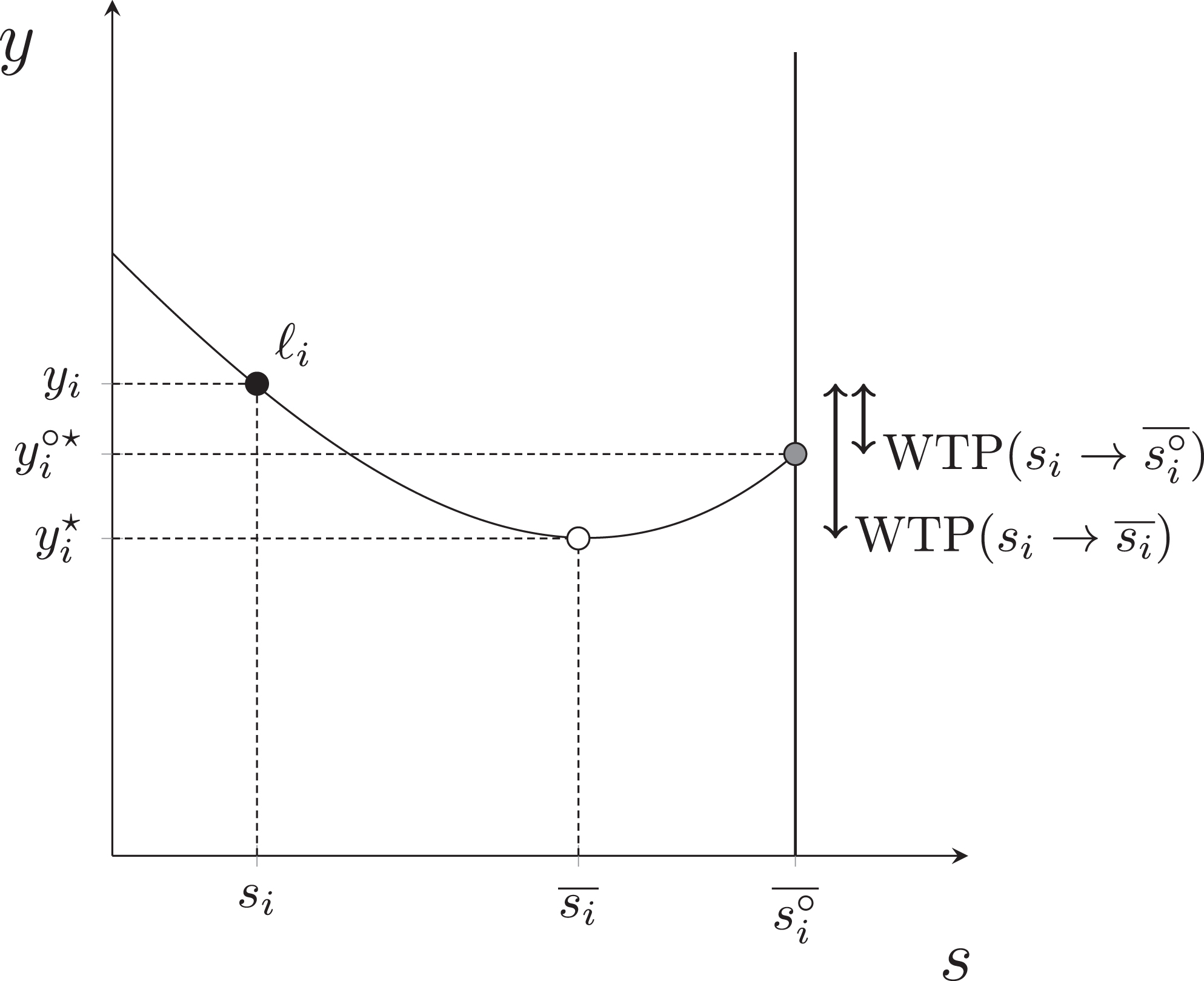
Nonmonotonic preferences over social interactions
Nonmonotonic preferences over social interactions
A more fundamental challenge in eliciting equivalent income is raised by insights from behavioral economics. Accumulating evidence suggests that respondents often construct rather than retrieve well-defined preferences during the elicitation process, especially when faced with goods they have little prior experience with. This constructive process is highly sensitive to contextual cues within the survey, such as anchors and question framing (Lichtenstein and Slovic, 2006b). Payne et al. (2000) argue therefore that stated preference practitioners should view themselves as architects, aiding respondents in constructing “defensible” preferences, rather than as archaeologists unearthing pre-existing preferences.
This constructive view raises two challenges for stated preference researchers. The first is to establish the “best possible” context for respondents to elicit preferences. There is an ongoing debate within the field on this context, which we do not attempt to resolve here. Nevertheless, previous calls for a more constructive approach to contingent valuation, for instance via the use of multiattribute utility theory and decision analysis (Gregory et al., 1993), seem to have fallen short within the field in favor of shorter and more efficient multiattribute methods, such as discrete choice experiments.
The second challenge is ensuring that the theoretical concept being elicited is adaptable enough to accommodate context-dependent preferences (Bernheim, 2021). The equivalent income approach can account for context dependency to some extent by relaxing the completeness assumption (Fleurbaey and Schokkaert, 2013). This essentially implies that if A is preferred over B in one genuine choice context, but B is preferred over A in another, we lack sufficient information to establish a definitive ranking between A and B. Some studies have demonstrated how this can be operationalized using nonparametric techniques (Decancq and Nys, 2021; Burone and Decancq, 2023).
Avenues for future research
Based on this discussion, we propose several promising avenues for future research on equivalent incomes. First, there are variations of existing methods that have been relatively unexplored within the literature on equivalent income and well-being measurement more broadly:
-
Nonparametric methods: Methods like the ABDC approach could be extended to accommodate multiple nonmonetary dimensions. This is relatively straightforward for measuring well-being directly, as introducing additional dimensions does not require a greater number of choice sets than those currently used. Indeed, researchers would only need to elicit the equivalent income itself: the point that is the intersection between the indifference surface and a reference vector of dimensions (see, e.g., Burone and Decancq, 2023). However, challenges may arise with the curse of dimensionality if the objective is to estimate marginal rates of substitution or entire indifference maps.
-
Pivot designs: To our knowledge, aside from the small-scale study by Abasolo et al. (2018), choice experiments have not been widely employed to elicit equivalent income. This may reflect concerns that these methods do not yield individual-level preferences, a limitation shared by the life satisfaction method, which has nonetheless seen broader application in the literature. Future research could explore the potential of pivot designs. Typically, discrete choice experiments present alternatives preselected by the researcher, assuming that all individuals face the same choice situations. This may, however, be suboptimal from cognitive and contextual standpoints. For instance, respondents may struggle to relate to hypothetical scenarios far removed from their own experiences. Pivot designs, which have been used to reduce cognitive load and enhance realism in discrete choice experiments (see Rose et al., 2008), involve first identifying a respondent-specific reference alternative (e.g., their actual life situation). Attributes in the choice situations are then generated relative to this reference alternative (i.e., pivoted). For equivalent income elicitation, hypothetical life situations could be pivoted around respondents’ actual life situations. This follows a similar approach taken in contingent valuation studies on equivalent income, which compare respondents’ actual life situation to a reference situation. We foresee two advantages here: first, this approach allows efficient elicitation of marginal rates of substitution, thereby avoiding the curse of dimensionality; second, with careful experimental design, equivalent income could also be estimated nonparametrically.
-
Contingent rating: Traditional applications of conjoint analysis may conflict with the assumptions of equivalent income, but some variants could leverage the ordinal nature of respondents’ ratings. For instance, as proposed by Benjamin et al. (2017), individuals could be asked to predict their life satisfaction levels in various hypothetical scenarios. Marginal rates of substitution could then be estimated for the dimensions within these scenarios. This method extends the life satisfaction approach discussed earlier, relying on the same core assumption – namely, that ordinal preferences can be inferred from stated life satisfaction scores, known as the consistency assumption. Equivalent incomes could also be estimated nonparametrically based on these scores.
-
Constructive preferences: Developing elicitation techniques that aid respondents in forming their preferences represents a particularly promising area, with both empirical and ethical benefits. Empirically, preference estimations may be more robust when respondents are supported in refining incomplete preferences and mitigating cognitive biases. Ethically, these techniques are likely to yield preferences that are more authentic and thus more deserving of consideration in policy applications. This will be the focus of a follow-up paper.
Additionally, mixed surveys that combine and compare different preference elicitation techniques may yield valuable insights. For instance, Burone and Decancq (2023) administered both ABDC and contingent valuation methods to respondents in varying sequences, comparing responses both between and within groups. They found that respondents with precise (complete) preferences gave consistent answers across methods, while those with more incomplete preferences showed less consistency. This suggests that combining different approaches may be an effective strategy for helping respondents refine their preferences during the survey process.
Conclusion
While preference elicitation methods are increasingly dominated by multiattribute approaches, especially discrete choice experiments, this paper argues that the measurement of well-being, particularly through equivalent income, warrants a broader exploration of preference elicitation methods. Estimating the distribution of well-being with a preference-based measure naturally suggests methods that capture individual-level preference heterogeneity, with contingent valuation offering key advantages in this respect. Yet, even methods limited to group-level estimates of preferences are valuable, especially if they allow us to infer preference distributions. Clearly, the limitations of the different methods leave ample room for methodological innovation. We have discussed some promising avenues in this review.
The need for robust preference estimates goes beyond academic interest. Policy decisions may be indirectly shaped by population preferences when citizens support policy platforms in democratic elections. However, this is no substitute for directly tailoring policies to the diverse life situations and preferences within the population. Citizens may base their policy preferences on broad (mis)information and vote accordingly, but their personal preferences on trade-offs between dimensions like income, health, employment, social status, and relationships are invaluable for decisions on budget allocation and program prioritization. Making such information more widely available would provide critical information for public debate and policy deliberation. Additionally, well-being measures like equivalent income, which account for the effect of correlated disadvantages across life dimensions and the importance individuals give to these dimensions, can offer essential insight into the distributive effects of policies. Developing preference elicitation methods to supply the public debate with this crucial information should therefore be a priority.
References
- Abasolo, I., C. Sandelind, E. Schokkaert, K. Stevens, and A. Tsuchiya (2018). “Operationalising equivalent consumption through stated preferences: A pilot Study in two Parts,” CWiPP Working Paper Series.
- Adler, M. D. (2019). Measuring Social Welfare: An Introduction, Oxford University Press.
- Adler, M. D. and P. Dolan (2008). “Introducing a ‘different lives’ approach to the valuation of health and well-being,” U of Penn, Inst for Law & Econ Research Paper.
- Adler, M. D., P. Dolan, and G. Kavetsos (2017). “Would you choose to be happy? Tradeoffs between happiness and the other dimensions of life in a large population survey,” Journal of Economic Behavior & Organization, 139, 60–73.
- Adler, M. D. and M. Fleurbaey (2016). The Oxford Handbook of Well-Being and Public Policy, Oxford University Press.
- Akay, A., O. Bargain, and H. X. Jara (2020). “Fair welfare comparisons with heterogeneous tastes: subjective versus revealed preferences,” Social Choice and Welfare, 55, 51–84.
- Akay, A., O. B. Bargain, and H. X. Jara (2023). “Experienced versus decision utility: large-scale comparison for income–leisure preferences,” The Scandinavian Journal of Economics, 125, 823–859.
- Alberini, A. (2019). “Revealed versus stated preferences: what have we learned about valuation and behavior?” Review of Environmental Economics and Policy.
- Arrow, K., R. Solow, P. R. Portney, E. E. Leamer, R. Radner, H. Schuman, et al. (1993). “Report of the NOAA panel on contingent valuation,” Federal Register, 58, 4601–4614.
- Atkinson, G. and S. Mourato (2015). “Cost-benefit analysis and the environment,” OECD Environment Working Papers No. 97, OECD Publishing, Paris.
- Attema, A. E. and W. B. Brouwer (2013). “In search of a preferred preference elicitation method: A test of the internal consistency of choice and matching tasks,” Journal of Economic Psychology, 39, 126–140.
- Bargain, O., A. Decoster, M. Dolls, D. Neumann, A. Peichl, and S. Siegloch (2013). “Welfare, labor supply and heterogeneous preferences: evidence for Europe and the US,” Social Choice and Welfare, 41, 789–817.
- Bateman, I. J., R. T. Carson, B. Day, M. Hanemann, N. Hanley, T. Hett, M. Jones-Lee, G. Loomes, S. Mourato, E. Ozdemiroglu, D. Pearce, R. Sugden, and J. Swanson (2002). Economic Valuation with Stated Preference Techniques: A Manual, Edward Elgar Cheltenham.
- Becker, G. M., M. H. DeGroot, and J. Marschak (1964). “Measuring utility by a single-response sequential method,” Behavioral Science, 9, 226–232.
- Beegle, K., K. Himelein, and M. Ravallion (2012). “Frame-of-reference bias in subjective welfare,” Journal of Economic Behavior & Organization, 81, 556–570.
- Benjamin, D. J., K. Cooper, O. Heffetz, and M. Kimball (2017). “Challenges in constructing a survey-based well-being index,” American Economic Review, 107, 81–85.
- Benjamin, D. J., K. Cooper, O. Heffetz, and M. Kimball (2023a). “From happiness data to economic conclusions,” Annual Review of Economics, 16.
- Benjamin, D. J., K. Cooper, O. Heffetz, M. S. Kimball, and J. Zhou (2023b). “Adjusting for scale-use heterogeneity in self-reported well-being,” Working Paper w31728, National Bureau of Economic Research.
- Benjamin, D. J., J. Debnam Guzman, M. Fleurbaey, O. Heffetz, and M. Kimball (2023c). “What do happiness data mean? Theory and survey evidence,” Journal of the European Economic Association, 21, 2377–2412.
- Benjamin, D. J., O. Heffetz, M. Kimball, and N. Szembrot (2014a). “Beyond happiness and satisfaction: Toward well-being indices based on stated preference,” American Economic Review, 104, 2698–2735.
- Benjamin, D. J., O. Heffetz, M. S. Kimball, and A. Rees-Jones (2012). “What do you think would make you happier? What do you think you would choose?” American Economic Review, 102, 2083–2110.
- Benjamin, D. J., O. Heffetz, M. S. Kimball, and A. Rees-Jones (2014b). “Can marginal rates of substitution be inferred from happiness data? Evidence from residency choices,” American Economic Review, 104, 3498–3528.
- Bernheim, B. D. (2016). “The good, the bad, and the ugly: A unified approach to behavioral welfare economics,” Journal of Benefit-Cost Analysis, 7, 12–68.
- Bernheim, B. D. (2021). “In defense of behavioral welfare economics,” Journal of Economic Methodology, 28, 385–400.
- Bijlenga, D., G. J. Bonsel, and E. Birnie (2011). “Eliciting willingness to pay in obstetrics: Comparing a direct and an indirect valuation method for complex health outcomes,” Health Economics, 20, 1392–1406.
- Bishop, R. C. and K. J. Boyle (2019). “Reliability and validity in nonmarket valuation,” Environmental and Resource Economics, 72, 559–582.
- Boarini, R., M. Fleurbaey, F. Murtin, and P. Schreyer (2022). “Well-being during the Great Recession: New evidence from a measure of multi-dimensional living standards with heterogeneous preferences,” The Scandinavian Journal of Economics, 124, 104–138.
- Bond, T. N. and K. Lang (2019). “The sad truth about happiness scales,” Journal of Political Economy, 127, 1629–1640.
- Bosmans, K., K. Decancq, and E. Ooghe (2018). “Who’s afraid of aggregating money metrics?” Theoretical Economics, 13, 467–484.
- Burone, S. and K. Decancq (2023). “Measuring multidimensional well-being when preferences differ: a non-parametric approach,” MIMEO, https://www.ecineq.org/wp-content/uploads/2023/06/EcineqAMSE-267.pdf
- Capéau, B., L. Cherchye, K. Decancq, A. Decoster, B. D. Rock, F. Maniquet, A. Nys, G. Périlleux, E. Ramaekers, Z. Rongé, et al. (2020). “Who has the lowest levels of well-being?” Well-being in Belgium: Beyond Happiness and Income, 175–181.
- Carson, R. T. (2012). “Contingent valuation: A practical alternative when prices aren’t available,” Journal of Economic Perspectives, 26, 27–42.
- Carson, R. T. and T. Groves (2007). “Incentive and informational properties of preference questions,” Environmental and Resource Economics, 37, 181–210.
- Cavapozzi, D., W. Han, and R. Miniaci (2015). “Alternative weighting structures for multidimensional poverty assessment,” The Journal of Economic Inequality, 13, 425–447.
- Champ, P. A. and R. C. Bishop (2006). “Is willingness to pay for a public good sensitive to the elicitation format?” Land Economics, 82, 162–173.
- Champonnois, V., O. Chanel, and K. Makhloufi (2018). “Reducing the anchoring bias in multiple question CV surveys,” Journal of Choice Modelling, 28, 1–9.
- Chanel, O., K. Makhloufi, and M. Abu-Zaineh (2017). “Can a circular payment card format effectively elicit preferences? Evidence from a survey on a mandatory health insurance scheme in Tunisia,” Applied Health Economics and Health Policy, 15, 385–398.
- Clark, A. E. and A. J. Oswald (2002). “A simple statistical method for measuring how life events affect happiness,” International Journal of Epidemiology, 31, 1139–1144.
- Cookson, R., I. Skarda, O. Cotton-Barratt, M. Adler, M. Asaria, and T. Ord (2021). “Quality adjusted life years based on health and consumption: A summary wellbeing measure for cross-sectoral economic evaluation,” Health Economics, 30, 70–85.
- Cummings, R. G. and L. O. Taylor (1999). “Unbiased value estimates for environmental goods: A cheap talk design for the contingent valuation method,” American Economic Review, 89, 649–665.
- Danyliv, A., M. Pavlova, I. Gryga, and W. Groot (2012). “Willingness to pay for physician services: Comparing estimates from a discrete choice experiment and contingent valuation,” Society and Economy, 34, 339–357.
- Deaton, A. (1979). “The distance function in consumer behaviour with applications to index numbers and optimal taxation,” The Review of Economic Studies, 46, 391–405.
- Deaton, A., J. Fortson, and R. Tortora (2009). “Life (evaluation), HIV/AIDS, and death in Africa,” Tech. rep., National Bureau of Economic Research.
- Decancq, K., M. Fleurbaey, and F. Maniquet (2019). “Multidimensional poverty measurement with individual preferences,” The Journal of Economic Inequality, 17, 29–49.
- Decancq, K., M. Fleurbaey, and E. Schokkaert (2015a). “Happiness, equivalent incomes and respect for individual preferences,” Economica, 82, 1082–1106.
- Decancq, K., M. Fleurbaey, and E. Schokkaert (2015b). Inequality, Income and Wellbeing. Handbook of Income Distribution, Vol. 2A. eds. A. Atkinson, and F. Bourguignon, 67–140.
- Decancq, K., M. Fleurbaey, and E. Schokkaert (2017). “Wellbeing Inequality and Preference Heterogeneity,” Economica, 84, 210–238.
- Decancq, K. and A. Michiels (2017). “Measuring successful aging with respect for preferences of older persons,” The Journals of Gerontology: Series B, 74, 364–372.
- Decancq, K. and D. Neumann (2016). “Does the choice of well-being measure matter empirically? An illustration with German data,” in Oxford Handbook of Well-Being and Public Policy, ed. Matthew Adler and Marc Fleurbaey, Oxford University Press, 553–587.
- Decancq, K. and A. Nys (2021). “Non-parametric well-being comparisons,” European Economic Review, 133, 103666.
- Decancq, K., J. Olivera, and E. Schokkaert (2025). “Ethnic differences and preference heterogeneity: assessing social pensions in Peru,” Development Studies Research, 12, 2443233.
- Decancq, K. and S. Panagamuwa Gamage (2025). “Converging lives? Measuring and understanding well-being inequality in the European Union,” Mimeo.
- Decancq, K. and E. Schokkaert (2016). “Beyond GDP: Using equivalent incomes to measure well-being in Europe,” Social Indicators Research, 126, 21–55.
- Decancq, K., E. Schokkaert, and B. Zuluaga (2020). “Implementing the capability approach with respect for individual valuations: An illustration with Colombian data,” in The Cambridge University Press Handbook of the Capability Approach, ed. Enrica Chiappero-Martinetti, Siddiq Osmani, and Mozaffar Qizilbash, Cambridge University Press, 307–332.
- Decoster, A. M. and P. Haan (2015). “Empirical welfare analysis with preference heterogeneity,” International Tax and Public Finance, 22, 224–251.
- Defloor, B., E. Verhofstadt, and L. Van Ootegem (2017). “The influence of preference information on equivalent income,” Social Indicators Research, 131, 489–507.
- Desvousges, W., K. Mathews, and K. Train (2012). “Adequate responsiveness to scope in contingent valuation,” Ecological Economics, 84, 121–128.
- Desvousges, W., K. Mathews, and K. Train (2016). “From curious to pragmatically curious: comment on ‘From hopeless to curious? Thoughts on Hausman’s ’dubious to hopeless’ critique of contingent valuation,’ ” Applied Economic Perspectives and Policy, 38, 174–182.
- Deyshappriya, N. R. and S. Feeny (2021). “Weighting the dimensions of the Multidimensional Poverty Index: Findings from Sri Lanka,” Social Indicators Research, 1–19.
- Dhillon, A. and J.-F. Mertens (1999). “Relative utilitarianism,” Econometrica, 67, 471–498.
- Diamond, P. A. and J. A. Hausman (1994). “Contingent valuation: Is some number better than no number?” Journal of Economic Perspectives, 8, 45–64.
- Dolan, P. and R. Metcalfe (2008). “Comparing willingness-to-pay and subjective well-being in the context of non-market goods,” Centre for Economic Performance Discussion Paper 890.
- Dubourg and G. Loomes (1997). “Imprecise preferences and survey design in contingent valuation,” Economica, 64, 681–702.
- Ferrer-i-Carbonell, A. and B. M. Van Praag (2002). “The subjective costs of health losses due to chronic diseases. An alternative model for monetary appraisal,” Health Economics, 11, 709–722.
- Finkelstein, A., E. F. Luttmer, and M. J. Notowidigdo (2013). “What good is wealth without health? The effect of health on the marginal utility of consumption,” Journal of the European Economic Association, 11, 221–258.
- Fleurbaey, M. (2009). “Beyond GDP: The quest for a measure of social welfare,” Journal of Economic Literature, 47, 1029–1075.
- Fleurbaey, M. and D. Blanchet (2013). Beyond GDP: Measuring Welfare and Assessing Sustainability, Oxford UniversityPress.
- Fleurbaey, M. and G. Gaulier (2009). “International comparisons of living standards by equivalent incomes,” Scandinavian Journal of Economics, 111, 597–624.
- Fleurbaey, M., S. Luchini, C. Muller, and E. Schokkaert (2013). “Equivalent income and fair evaluation of health care,” Health Economics, 22, 711–729.
- Fleurbaey, M. and F. Maniquet (2011). A Theory of Fairness and Social Welfare, vol.48, Cambridge University Press.
- Fleurbaey, M. and E. Schokkaert (2013). “Behavioral welfare economics and redistribution,” American Economic Journal: Microeconomics, 5, 180–205.
- Fleurbaey, M. and H. Schwandt (2016). “Do people seek to maximize their subjective well-being?” CEP Discussion Paper 1391, London School of Economics and Political Science, Centre for Economic Performance, London.
- Fleurbaey, M. and K. Tadenuma (2014). “Universal social orderings: An integrated theory of policy evaluation, inter-society comparisons, and interpersonal comparisons,” Review of Economic Studies, 81, 1071–1101.
- Foster, H. and J. Burrows (2017). “Hypothetical bias: A new meta-analysis,” in Contingent Valuation of Environmental Goods, Edward Elgar Publishing, 270–291.
- Fujiwara, D. (2021). “Incorporating life satisfaction in discrete choice experiments to estimate well-being values for non-market goods,” Simetrica-Jacobs Research Paper.
- Gregory, R., S. Lichtenstein, and P. Slovic (1993). “Valuing environmental resources: A constructive approach,” Journal of Risk and Uncertainty, 7, 177–197.
- Gregory, R. S. (2000). “Valuing environmental policy options: A case study comparison of multiattribute and contingent valuation survey methods,” Land Economics, 151–173.
- Haab, T. C., M. G. Interis, D. R. Petrolia, and J. C. Whitehead (2013). “From hopeless to curious? Thoughts on Hausman’s ‘dubious to hopeless’ critique of contingent valuation,” Applied Economic Perspectives and Policy, 35, 593–612.
- Haab, T. C., M. G. Interis, D. R. Petrolia, and J. C. Whitehead (2016). “Interesting questions worthy of further study: Our reply to Desvousges, Mathews, and Train’s (2015) comment on our thoughts (2013) on Hausman’s (2012) update of Diamond and Hausman’s (1994) critique of contingent valuation,” Applied Economic Perspectives and Policy, 38, 183–189.
- Haghani, M., M. C. Bliemer, J. M. Rose, H. Oppewal, and E. Lancsar (2021). “Hypothetical bias in stated choice experiments: Part I. Macro-scale analysis of literature and integrative synthesis of empirical evidence from applied economics, experimental psychology and neuroimaging,” Journal of Choice Modelling, 41, 100309.
- Hanemann, M., J. Loomis, and B. Kanninen (1991). “Statistical efficiency of double-bounded dichotomous choice contingent valuation,” American Journal of Agricultural Economics, 73, 1255–1263.
- Hanemann, W. M. (1984). “Welfare evaluations in contingent valuation experiments with discrete responses,” American Journal of Agricultural Economics, 66, 332–341.
- Hanley, N., S. Mourato, and R. E. Wright (2001). “Choice modelling approaches: a superior alternative for environmental valuatioin?” Journal of Economic Surveys, 15, 435–462.
- Hausman, D. M. (2011). Preference, Value, Choice, and Welfare, Cambridge University Press.
- Hausman, J. (2012). “Contingent valuation: From dubious to hopeless,” Journal of Economic Perspectives, 26, 43–56.
- Heffetz, O. and M. Rabin (2013). “Conclusions regarding cross-group differences in happiness depend on difficulty of reaching respondents,” American Economic Review, 103, 3001–3021.
- Himmler, S., J. Stöckel, J. van Exel, and W. B. Brouwer (2021). “The value of health: Empirical issues when estimating the monetary value of a quality-adjusted life year based on well-being data,” Health Economics, 30, 1849–1870.
- Hole, A. R. (2008). “Modelling heterogeneity in patients’ preferences for the attributes of a general practitioner appointment,” Journal of Health Economics, 27, 1078–1094.
- Hole, A. R. (2011). “A discrete choice model with endogenous attribute attendance,” Economics Letters, 110, 203–205.
- Humphreys, B. R., B. K. Johnson, and J. C. Whitehead (2020). “Validity and reliability of contingent valuation and life satisfaction measures of welfare: an application to the value of national Olympic success,” Southern Economic Journal, 87, 316–330.
- Jacquemet, N., R.-V. Joule, S. Luchini, and J. F. Shogren (2013). “Preference elicitation under oath,” Journal of Environmental Economics and Management, 65, 110–132.
- Jara, H. X. and E. Schokkaert (2017). “Putting measures of individual well-being to use for ex-ante policy evaluation,” The Journal of Economic Inequality, 15, 421–440.
- Johnson, F. R., E. Lancsar, D. Marshall, V. Kilambi, A. Mühlbacher, D. A. Regier, B. W. Bresnahan, B. Kanninen, and J. F. Bridges (2013). “Constructing experimental designs for discrete-choice experiments: Report of the ISPOR conjoint analysis experimental design good research practices task force,” Value in Health, 16, 3–13.
- Johnson, T., P. Kulesa, Y. I. Cho, and S. Shavitt (2005). “The relation between culture and response styles: Evidence from 19 countries,” Journal of Cross-cultural Psychology, 36, 264–277.
- Johnston, R. J., K. J. Boyle, W. Adamowicz, J. Bennett, R. Brouwer, T. A. Cameron, W. M. Hanemann, N. Hanley, M. Ryan, R. Scarpa, et al. (2017). “Contemporary guidance for stated preference studies,” Journal of the Association of Environmental and Resource Economists, 4, 319–405.
- Jones, C. I. and P. J. Klenow (2016). “Beyond GDP? Welfare across countries and time,” American Economic Review, 106, 2426–57.
- Kaiser, C. and A. J. Oswald (2022). “Inequality, well-being, and the problem of the unknown reporting function,” Proceedings of the National Academy of Sciences, 119, e2217750119.
- King, G., C. J. Murray, J. A. Salomon, and A. Tandon (2004). “Enhancing the validity and cross-cultural comparability of measurement in survey research,” American Political Science Review, 98, 191–207.
- Kling, C. L., D. J. Phaneuf, and J. Zhao (2012). “From Exxon to BP: Has some number become better than no number?” Journal of Economic Perspectives, 26, 3–26.
- Knight, J., S. Lina, and R. Gunatilaka (2009). “Subjective well-being and its determinants in rural China,” China Economic Review, 20, 635–649.
- Kuhfeld, W. F. (2003). Marketing Research Methods in SAS. Citeseer.
- Kwak, S.-J., S.-H. Yoo, and T.-Y. Kim (2001). “A constructive approach to air-quality valuation in Korea,” Ecological Economics, 38, 327–344.
- Lancsar, E. and J. Louviere (2006). “Deleting ‘irrational’ responses from discrete choice experiments: a case of investigating or imposing preferences?” Health Economics, 15, 797–811.
- Layard, R., G. Mayraz, and S. Nickell (2008). “The marginal utility of income,” Journal of Public Economics, 92, 1846–1857.
- Ledić, M. and I. Rubil (2019). “Decomposing the difference between well-being inequality and income inequality: Method and application,” in What Drives Inequality?, Emerald Publishing Limited, vol. 27, 105–122.
- Ledić, M. and I. Rubil (2021). “Beyond wage gap, towards job quality gap: The role of inter-group differences in wages, non-wage job dimensions, and preferences,” Social Indicators Research, 155, 523–561.
- Leitner, L. (2024). “Imprecision in the estimation of willingness to pay using subjective well-being data,” Journal of Happiness Studies, 25, 1–40.
- Lichtenstein, S. and P. Slovic (2006a). The Construction of Preference, Cambridge University Press.
- Lichtenstein, S. and P. Slovic (2006b). The Construction of Preference, Cambridge University Press Cambridge.
- List, J. A. and C. A. Gallet (2001). “What experimental protocol influence disparities between actual and hypothetical stated values?” Environmental and Resource Economics, 20, 241–254.
- Loomis, J. (2011). “What’s to know about hypothetical bias in stated preference valuation studies?” Journal of Economic Surveys, 25, 363–370.
- Luechinger, S. (2009). “Valuing air quality using the life satisfaction approach,” The Economic Journal, 119, 482–515.
- MacCrimmon, K. R. and M. Toda (1969). “The experimental determination of indifference curves,” The Review of Economic Studies, 36, 433–451.
- Magat, W. A., W. K. Viscusi, and J. Huber (1988). “Paired comparison and contingent valuation approaches to morbidity risk valuation,” Journal of Environmental Economics and Management, 15, 395–411.
- Masterman, C. and W. K. Viscusi (2018). “The income elasticity of global values of a statistical life: Stated preference evidence,” Journal of Benefit Cost Analysis, 9, 407–434.
- McFadden, D. and K. Train (2000). “Mixed MNL models for discrete response,” Journal of applied Econometrics, 15, 447–470.
- McFadden, D.et al. (1973). “Conditional logit analysis of qualitative choice behavior,” in Frontiers in Econometrics, ed. P. Zarembka, 105–142, Academic Press.
- McGillivray, M., S. Feeny, P. Hansen, S. Knowles, and F. Ombler (2023). “What are valid weights for the Human Development Index? A discrete choice experiment for the United Kingdom,” Social Indicators Research, 165, 679–694.
- Moore, S. and J. P. Shepherd (2006). “The cost of fear: Shadow pricing the intangible costs of crime,” Applied Economics, 38, 293–300.
- Mori, Y. and N. Sakamoto (2024). “Does the choice of well-being measures matter in respecting human dignity? empirical results from an Indian slum survey,” in Dignity, Freedom and Justice, Springer Nature SingaporeSingapore, 229–258.
- Moscati, I. (2007). “Early experiments in consumer demand Theory: 1930-1970,” History of Political Economy, 39, 359–401.
- Murphy, J. J., P. G. Allen, T. H. Stevens, and D. Weatherhead (2005). “A meta-analysis of hypothetical bias in stated preference valuation,” Environmental and Resource Economics, 30, 313–325.
- Murtin, F., R. Boarini, J. C. Cordoba, and M. Ripoll (2017). “Beyond GDP: Is there a law of one shadow price?” European Economic Review, 100, 390–411.
- Nunes, P. A. and E. Schokkaert (2003). “Identifying the warm glow effect in contingent valuation,” Journal of Environmental Economics and Management, 45, 231–245.
- Onder, H., P. Pestieau, and G. Ponthiere (2025). “Equivalent income versus equivalent lifetime: Does the metric matter?” Journal of Demographic Economics, 91, 210–239.
- Orlowski, J. and P. Wicker (2015). “The monetary value of social capital,” Journal of Behavioral and Experimental Economics, 57, 26–36.
- Oswald, A. J. (2008). “On the curvature of the reporting function from objective reality to subjective feelings,” Economics Letters, 100, 369–372.
- Oswald, A. J. and N. Powdthavee (2008). “Death, happiness, and the calculation of compensatory damages,” The Journal of Legal Studies, 37, S217–S251.
- Payne, J. W., J. R. Bettman, D. A. Schkade, N. Schwarz, and R. Gregory (2000). “Measuring constructed preferences: Towards a building code,” Elicitation of Preferences, 243–275.
- Pazner, E. A. and D. Schmeidler (1978). “Egalitarian equivalent allocations: A new concept of economic equity,” The Quarterly Journal of Economics, 92, 671–687.
- Penn, J. M. and W. Hu (2018). “Understanding hypothetical bias: An enhanced meta-analysis,” American Journal of Agricultural Economics, 100, 1186–1206.
- Pinto-Prades, J. L., F. I. Sánchez-Martínez, J. M. Abellán-Perpiñán, and J. E. Martínez-Pérez (2018). “Reducing preference reversals: The role of preference imprecision and nontransparent methods,” Health Economics, 27, 1230–1246.
- Portney, P. R. (1994). “The contingent valuation debate: Why economists should care,” Journal of Economic Perspectives, 8, 3–17.
- Powdthavee, N. (2008). “Putting a price tag on friends, relatives, and neighbours: Using surveys of life satisfaction to value social relationships,” The Journal of Socio-Economics, 37, 1459–1480.
- Powdthavee, N. (2010). “How much does money really matter? Estimating the causal effects of income on happiness,” Empirical Economics, 39, 77–92.
- Rakotonarivo, O. S., M. Schaafsma, and N. Hockley (2016). “A systematic review of the reliability and validity of discrete choice experiments in valuing non-market environmental goods,” Journal of Environmental Management, 183, 98–109.
- Ravallion, M., K. Himelein, and K. Beegle (2016). “Can subjective questions on economic welfare be trusted?” Economic Development and Cultural Change, 64, 697–726.
- Roe, B., K. J. Boyle, and M. F. Teisl (1996). “Using conjoint analysis to derive estimates of compensating variation,” Journal of Environmental Economics and Management, 31, 145–159.
- Rose, J. M., M. C. Bliemer, D. A. Hensher, and A. T. Collins (2008). “Designing efficient stated choice experiments in the presence of reference alternatives,” Transportation Research Part B: Methodological, 42, 395–406.
- Russell, C., V. Dale, J. Lee, M. H. Jensen, M. Kane, and R. Gregory (2001). “Experimenting with multi-attribute utility survey methods in a multi-dimensional valuation problem,” Ecological Economics, 36, 87–108.
- Ryan, M., D. A. Scott, and C. Donaldson (2004). “Valuing health care using willingness to pay: A comparison of the payment card and dichotomous choice methods,” Journal of Health Economics, 23, 237–258.
- Ryan, M. and V. Watson (2009). “Comparing welfare estimates from payment card contingent valuation and discrete choice experiments,” Health Economics, 18, 389–401.
- Samson, A.-L., E. Schokkaert, C. Thébaut, B. Dormont, M. Fleurbaey, S. Luchini, and C. Van de Voorde (2018). “Fairness in cost-benefit analysis: A methodology for health technology assessment,” Health Economics, 27, 102–114.
- Samuelson, P. A. (1974). “Complementarity: An essay on the 40th anniversary of the Hicks-Allen revolution in demand theory,” Journal of Economic Literature, 12, 1255–1289.
- Schokkaert, E., C. Van de Voorde, B. Dormont, M. Fleurbaey, S. Luchini, A.-L. Samson, and C. Thébaut (2013). “Equity in health and equivalent incomes,” in Health and Inequality, Emerald Group Publishing Limited, 131–156.
- Schokkaert, E., L. Van Ootegem, and E. Verhofstadt (2011). “Preferences and subjective satisfaction: Measuring well-being on the job for policy evaluation,” CESifo Economic Studies, 57, 683–714.
- Sen, A. K. (1985). Commodities and Capabilities, North-Holland.
- Stiglitz, J., A. Sen, J.-P. Fitoussi, et al. (2009). “The measurement of economic performance and social progress revisited,” Reflections and Overview. Commission on the Measurement of Economic Performance and Social Progress, Paris.
- Ta, A., B. Van Landeghem, and A. Tsuchiya (2024). “Eliciting public preferences across health and wellbeing dimensions: An equivalent income value set for SIPHER-7,” Health Economics, 33, 2723–2741.
- Thurstone, L. L. (1931). “The indifference function,” The Journal of Social Psychology, 2, 139–167.
- Train, K. and M. Weeks (2005). Discrete Choice Models in Preference Space and Willingness-to-Pay Space, Springer.
- Train, K. E. (2009). Discrete Choice Methods with Simulation, Cambridge University Press.
- Tversky, A., S. Sattath, and P. Slovic (1988). “Contingent weighting in judgment and choice,” Psychological Review, 95, 371.
- van der Pol, M., A. Shiell, F. Au, D. Johnston, and S. Tough (2008). “Convergent validity between a discrete choice experiment and a direct, open-ended method: Comparison of preferred attribute levels and willingness to pay estimates,” Social Science & Medicine, 67, 2043–2050.
- Van Loon, V. and K. Decancq (2022). “Using a factorial survey to estimate the relative importance of well-being dimensions according to older people: Insights from a repeated survey experiment in Flanders,” Innovation in Aging, 6, igac034.
- Van Loon, V. and K. Decancq (2024). “Well-BOA: Exploring a new preference-based instrument to compare well-being across older people,” Herman Deleeck Centre for Social Policy Working Paper Series 24/04.
- Varian, H. R. (1982). “The nonparametric approach to demand analysis,” Econometrica, 50, 945–973.
- Veneri, P. and F. Murtin (2019). “Where are the highest living standards? Measuring well-being and inclusiveness in OECD regions,” Regional Studies, 53, 657–666.
- Viscusi, W. K. and C. J. Masterman (2017). “Income elasticities and global values of a statistical life,” Journal of Benefit-Cost Analysis, 8, 226–250.
- Vossler, C. A. and E. Zawojska (2020). “Behavioral drivers or economic incentives? Toward a better understanding of elicitation effects in stated preference studies,” Journal of the Association of Environmental and Resource Economists, 7, 279–303.
- Wang, H. and D. Whittington (2005). “Measuring individuals’ valuation distributions using a stochastic payment card approach,” Ecological Economics, 55, 143–154.
- Watson, V., C. Dibben, M. Cox, I. Atherton, M. Sutton, and M. Ryan (2019). “Testing the expert based weights used in the UKs Index of Multiple Deprivation (IMD) against three preference-based Methods,” Social Indicators Research, 144, 1055–1074.
- Welsch, H. (2006). “Environment and happiness: Valuation of air pollution using life satisfaction data,” Ecological Economics, 58, 801–813.
- Welsh, M. P. and G. L. Poe (1998). “Elicitation effects in contingent valuation: Comparisons to a multiple bounded discrete choice approach,” Journal of Environmental Economics and Management, 36, 170–185.
- Whitehead, J. C. (2016). “Plausible responsiveness to scope in contingent valuation,” Ecological Economics, 128, 17–22.
- Yang, L. (2018). “Measuring well-being: A multidimensional index integrating subjective well-being and preferences,” Journal of Human Development and Capabilities, 19, 456–476.
- Yu, J., P. Goos, and M. Vandebroek (2011). “Individually adapted sequential Bayesian conjoint-choice designs in the presence of consumer heterogeneity,” International Journal of Research in Marketing, 28, 378–388.
Figures
The concept of equivalent income
The concept of equivalent income
A taxonomy of preference elicitation methods.
A taxonomy of preference elicitation methods.
Illustration of the ABDC method
Illustration of the ABDC method
Nonmonotonic preferences over social interactions
Nonmonotonic preferences over social interactions
Tables
| Mechanism | Example | Advantages | Disadvantages |
|---|---|---|---|
| Open-ended | • What is the maximum amount of income you would give up to obtain ? | • Straightforward question. • Avoids cues (no starting point/anchoring bias). • Provides WTP estimate for each respondent. |
• Large nonresponse rates (protest answers, zeros, outliers). • Cognitively challenging for respondents. |
| Payment card | • What is the maximum amount of income you would give up to obtain ? €0-10, €0-20,…, >€200? | • Avoids starting point bias (cards are laid before respondent). • Number of outliers (i.e., very large bids) may be reduced. • Provides interval coded WTP values at individual level. |
• Responses coded on an interval. • The width of the intervals and limits for the payment cards may lead to potential bias. |
| Referendum | • Single bounded: would you be willing to pay to obtain ? Yes/No • Double bounded: would you be willing to pay to obtain ? (e.g., if Yes, would you pay ; if No, would you pay ?) |
• Cognitively easier for respondents than open-ended. Only one value to consider. • Provides incentives for truthfully revealing preferences. • Minimizes non-response and outliers. • Provides interval coded WTP values at individual level. |
• Vulnerable to “yes-saying” (i.e., giving false affirmative answers). • Subject to starting point bias (i.e., WTP may be influenced by starting bid). • Statistically inefficient as each respondent is only asked one question or two questions (double bounded). |
| Bidding game | • Would you be willing to pay to obtain ? If Yes: interviewer keeps increasing bids until the respondent answers no. If No: interviewer keeps decreasing bids until respondent answers yes. | • Cognitively easier for respondents than open-ended. • Provides single or interval coded WTP values at the individual level. |
• Vulnerable to “yes-saying” (i.e., giving false affirmative answers). • Subject to anchoring bias (i.e., WTP may be influenced by starting bid). |
| Example | Advantages | Disadvantages |
|---|---|---|
| • Imagine two possible lives: your own and another . Which life would you choose? | • Elicitation of various points along the indifference curve, not just WTP. • Cognitively easier for respondents than open-ended questions. • Aligns with behavioral economic interpretations of the equivalent income. |
• Staring-point bias, preferences may be influenced by starting values. • WTP values are provided on an interval. • Many questions may be required to elicit indifference surfaces in multiple dimensions. |
| Method | Example | Advantages | Disadvantages |
|---|---|---|---|
| Discrete choice experiment | • Which life would you prefer? Please choose from the two options below. | • Mimics real-life decision-making processes. • Linked to RUT, welfare consistent estimates. • Useful for predicting choices or impacts of policy. |
• Respondents might find it difficult to make multiple choices in succession. • Only indicates ranking not strength of preference. |
| Rank-order choice experiment | • Please rank the following life situations according to your preference. | • Provides relative preference information, not just choice. • Linked to RUT, can provide welfare consistent estimates. • Useful for small samples as provides more information per respondent. |
• May be cognitively difficult to rank many alternatives at once. • Only indicates ranking not strength of preference • Requires more complex design and modelling techniques (e.g., rank-order logit). |
| Contingent rating | • On a scale of 0-10, please rate the following hypothetical life situations. | • Allows respondents to express their strength of preference. • Analysis relies on simple statistical techniques, e.g., OLS. |
• Relies on strong assumptions of cardinal and interpersonally comparable scale use. • Cognitively challenging to rate alternatives |
| Pairwise comparisons | • Which life would you prefer? Please indicate your strength of preference below. | • Reduces cognitive load by allowing respondents to rate two alternatives at a time. • Ratings can also be analyzed as implied choices. |
• Rating multiple pairs imposes larger cognitive load than discrete choice experiments |
| Theoretical objectives easier for estimating… | Preference heterogeneity at the level of… | |
|---|---|---|
| Contingent valuation | ||
| Open-ended | equivalent income | Individual |
| Referendum | equivalent income | Group |
| Payment cards | equivalent income | Individual |
| Bidding game | equivalent income | Individual |
| ABDC | equivalent income, indif. sets | Individual |
| Multiattribute methods | ||
| Discrete choice | MRS, indif. curves | Group |
| Ranking | MRS, indif. curves | Group |
| Contingent rating | MRS, indif. curves | Group |
| Pairwise comparisons | MRS, indif. curves | Group |
| Life satisfaction method | equivalent income, MRS, indif. curves | Group |