- VOL 1
- 2026
- research article
Abstract
This review summarizes research over the past two decades on human attitudes toward computationally “hard” problems. The focus is on the nature of uncertainty that computational complexity generates because humans do not have the cognitive capacity or the resources (time) to fully resolve the problems. Although decision theorists have traditionally labeled this type of uncertainty “ambiguity,” behavior under computational complexity shows that humans neither deal with it as prescribed in rational decision theory nor simply avoid it as in traditional accounts of ambiguity aversion. Instead, behavior (effort applied and performance reached) exhibits distinct features that can be rationalized using the theory of computational complexity, originally developed for electronic computers. Although the theory cannot decisively tell us which problems are most difficult, it does provide classifications that allow one to predict human performance and effort. The theory also identifies which instances of a problem are more difficult, and human performance and effort appear to align with this identification. Evidence is discussed that humans do not appear to allocate cognitive effort ex ante when faced with a hard choice. The absence of correlation between early neural signals and ex ante metrics of instance difficulty corroborates this finding. Finally, the heterogeneity in ways humans approach hard problems suggests that, collectively, much can be gained from incentive mechanisms that promote communication. Particular market designs appear to be extremely effective in helping participants make hard choices.
If you have ever attempted a crossword puzzle, you know that it is much harder to solve it from scratch than to verify a solution provided by someone else. […] The usual explanation for this difference of effort is that finding a solution to a crossword puzzle […] requires creative effort. [From Arora and Barak, 2009, chapter 2]
By Way of Introduction: Choice Consistency Versus Opportunism
How humans deal with uncertainty has been the subject of study for decades. Traditionally, this has been done through the lens of probability theory. The typical empirical paradigm is one where the experimenter randomly draws from an urn containing balls of different color. In a more sophisticated version of this probabilistic task, the two-armed bandit task, the agent is asked to decide which of two arms she prefers. The agent is allowed to explore before making up her mind. Absent specific information about the true payoff-generating process, the prescription is for the agent to start with some subjective beliefs about the chances that each of the arms pays and then use random draws made during exploration, together with Bayes’ law, to form a subjective posterior about the values of each of the arms, and choose the arm with the highest estimated value.
The resulting choice is optimal, in the sense that the agent’s choices will be consistent across several instantiations (instances) of the task. The agent is said to be “rational.” Among others, if she preferred the left arm, tried one more time the right arm, and produced an outcome that is below the expectation for the left arm without changing her beliefs about the risks, she must not switch preferences toward the right arm. Her choices are consistent with what she did in the past. She is “rational.”
Effectively, scholars of decision-making under uncertainty view the world as a gigantic casino full of multiarmed bandits. They teach that the rational approach in such a world is to start with subjective beliefs and valuations of outcomes, enhance their knowledge about the world by trial and error, and update their beliefs using Bayes’ law. If the updating is too demanding, efficient delta rules exist that approximate Bayes’ law (Wilson et al., 2013). If something is unknown, such as the true distance in kilometers between two cities, it should be treated as a random variable, a prior should be formed, and exploration by repeated measuring of the actual distance should lead to updates of one’s beliefs using Bayes’ law (Eisenführ et al., 2010).
The fact that most people would refuse to bet at all on a distance they do not know is considered “irrational.” It is even referred to as a paradox: the Ellsberg Paradox. The choice (not to bet) is categorized as a cognitive bias called ambiguity aversion or uncertainty aversion. That the distance is not random at all, and hence that there actually does not exist an objective prior to start updating with does not keep scholars from considering ambiguity aversion to be anomalous and hence shunned.
Here we consider situations where ambiguity arises because of complexity. Consider the graph coloring problem based on a map of the European Union depicted in figure 1(a), where more than 10 colors were used to distinguish member countries. Is it possible to color the countries with only four different hues such that no adjacent countries have the same color? You get 20 seconds to decide whether to bet for 100 euros that the answer is “yes.”
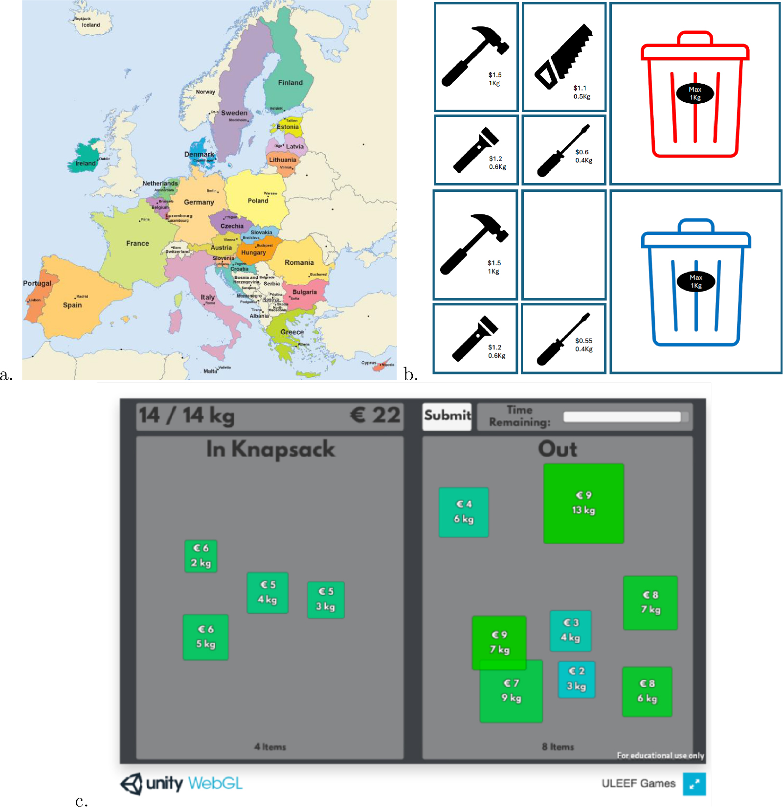
Figure 1. (a) Map of the European Union, downloaded from https://european-union.europa.eu/. The graph coloring task consists of finding whether member countries could be assigned colors so that no contiguous countries display the same color without using more than a limited number of colors, say four. In the map, more than 10 colors were used. (b) Which bin, if filled to capacity with a selection of the items depicted next to them, maximizes value? The greedy algorithm generates the wrong answer and hence does not maximize utility, even if it has good approximation properties in general. (c) Graphical interface of the knapsack problem optimization tasks used in experiments. Items from the right are to be moved into the knapsack to the left to maximize total value (in euros) without violating the capacity (expressed in kg). Reproduced from Bossaerts et al. (2024).
(a) Map of the European Union, downloaded from https://european-union.europa.eu/. The graph coloring task consists of finding whether member countries could be assigned colors so that no contiguous countries display the same color without using more than a limited number of colors, say four. In the map, more than 10 colors were used. (b) Which bin, if filled to capacity with a selection of the items depicted next to them, maximizes value? The greedy algorithm generates the wrong answer and hence does not maximize utility, even if it has good approximation properties in general. (c) Graphical interface of the knapsack problem optimization tasks used in experiments. Items from the right are to be moved into the knapsack to the left to maximize total value (in euros) without violating the capacity (expressed in kg). Reproduced from Bossaerts et al. (2024).
Note that the true chance is either zero (“It is impossible to color the map as requested with only four different hues”) or unity (“It is possible”). So, whichever prior the agent uses, it is necessarily subjective. One could try a random color pattern and then apply Bayes’ law. But Bayes’ law requires the likelihood function (i.e., the likelihood that some evidence emerges given that the true answer is “yes”), where evidence refers to outcomes such as: we randomly tried with four colors and exactly two adjacent countries ended up with the same color. There does not exist an objective way to calculate this chance, so the likelihood function we choose, like the prior, will be arbitrary.
The trial-and-error approach that can be so successful in traditional probabilistic tasks becomes absurd in the graph coloring problem. It would be similar to solving a jigsaw puzzle by repeated random throwing of its pieces on a table. It is true that, by chance, we would ultimately solve the puzzle, but we would have to try an inordinate number of times. If we decide to try only a finite number of times, we may end up with a really bad outcome: a picture that makes no sense.
Figure 1(b) provides another example. Imagine that we have to choose between two bins. Both have the same capacity: they can hold 1 Kg at most. Both bins come with valuable objects, which you get to keep, provided they fit in the bin. The red bin comes with four objects: a hammer, a saw, a flashlight, and a screwdriver, valued at $1.50, $1.10, $1.20, and $0.60, respectively, and weighing 1 Kg, 0.5 Kg, 0.6 Kg, and 0.4 Kg, respectively. The blue bin comes with only the hammer, flashlight, and screwdriver, and the screwdriver is worth only $0.55.
We could repeatedly and randomly fill bins with items, keeping track of the running maximum, until a finite stopping time. We could do this to obtain value estimates for both bins. But those estimates could be arbitrarily bad if, by chance, one fails to draw good solutions.
What about an alternative, which is to follow an algorithm (i.e., a sequence of—mostly if not always—deterministic steps that give us a good guess within a finite time)? Indeed, one could quickly evaluate how much each of the bins is worth by means of the greedy algorithm: sort the items in descending order of value over weight and fill the bin until capacity, skipping items when they would lead capacity to be violated. This algorithm is fast; it only requires sorting. It approximates the true solution well: it guarantees a solution with a value that is at least 50% of the optimal value. Applying this greedy algorithm, the red bin is estimated to be worth $1.70, while the blue bin is valued at $1.75. So the blue bin is chosen. But this choice is clearly not the optimal one. In fact, the obvious winner is the red bin, since it is always better to choose the option with more opportunities: the red bin offers everything the blue bin does, plus an extra item (a saw). In addition, the screwdriver is worth more in the red bin. So no “rational” agent would ever choose the blue bin.
The algorithmic approach is opportunistic, in the American sense of the term: “attentive to and ready to act on opportunities for personal gain or advancement” (from the Merriam-Webster Online Dictionary). It is attentive (uses a clever algorithm that guarantees a certain performance (50% of optimal value in the case of the bin-packing problem) and ready to act (it is fast). Contrast this to choice consistency: to be “rational” in choice, one does not have to be too attentive (randomly trying colors or items hardly requires cognitive effort), but it is slow (we would have to try a lot of times to be sure; if stopped in finite time, we could end up with an arbitrarily bad choice, by mere chance). Would one not prefer to be opportunistic here?
It is true that opportunism is often interpreted negatively, meaning that it advances one’s interest “without regard for principles” (Merriam-Webster Online Dictionary definition of “opportunism”). Opportunism can indeed violate principles—the principles of rationality, that is. In the bin-packing example of figure 1(b), the greedy algorithm violates a simple principle of rational choice: always choose the option with more possibilities, certainly if the corresponding values may be better.
The fact that the greedy algorithm causes irrational choice also implies that a utility function does not exist that, when optimized, could represent the agent’s choices. The decision theorist would call the choice “anomalous,” a cognitive bias, and perhaps refer to it as “simplicity seeking,” arguing that it is the result of “choice overload” (Reutskaja et al., 2018).
Note that the problem in figure 1(b) is essentially the standard consumer budget allocation problem of economic theory. The capacity of the bins can be thought of as the income of the consumer, the weights as the prices of the items, and the values as their utilities. The consumer can choose between two baskets and ends up choosing the simpler one, but unfortunately it provides inferior total utility. She does not optimize (but uses a good approximation algorithm).
Later in this paper, we consider experiments in which participants were asked to solve valuation problems of this type, called the bin packing problem, or the 0-1 knapsack problem (KP), with between 6 and 24 items, within a time limit of 25 seconds to 4 minutes. An example with 12 items is depicted in figure 1(c). In such situations, opportunism will trump consistency. It is true that the greedy algorithm requires harder thinking; more cognitive effort is required if only because the items have to be sorted. In the language of the previous quote from chapter 2 of Arora and Barak (2009), “creative effort” is required. Trying to quickly find random solutions may be easier; it certainly requires little effort. But the performance of trial and error happens to be worse than even that of the “brute force” algorithm, which is to list all feasible solutions and pick the best one. Even asymptotically (as the number of items increases), trial and error is no better.
What do our examples, the graph coloring and knapsack tasks, have in common? First, they are combinatorial rather than probabilistic: the task is to find the right combination of countries or items. In addition, the number of combinations increases exponentially in the number of countries that need to be colored or items that are available for the knapsack. Marginally moving one country (imagine if Switzerland joins the EU and Cyprus leaves) or changing the value or weight of one item may dramatically change the outcome. Second, the problems have in common that they require creative effort, in the sense that solving them is hard work while checking a solution is easy (see quote from chapter 2 from Arora and Barak, 2009). As a result, the two problems are considered computationally “hard” in a similar way, to the extent that they belong to an equivalence class referred to as NP-complete problems. This class contains many everyday problems, some of which are important for economics: budget allocation, attention allocation, production scheduling, routing, and so on.
NP-hard problems are thought to be computationally difficult. We ought to emphasize “thought,” in the following sense: humans have not yet found an algorithm that solves one of them in time that increases only as a polynomial in the input size (e.g., number of items in the KP; the number of countries in the map coloring problem). This then implies that the problems are hard even for electronic computers because they are programmed by humans.
Before proceeding, it may be worthwhile to point out that there are many different meanings of the term “complexity.” Here, it is referred to as the minimum number of computations needed to solve a problem (and hence resolve uncertainty) regardless of which algorithm is used, and, relatedly, the minimum memory that is required for any algorithm to solve a problem. Ryan Oprea and his collaborators have recently studied a very different kind of complexity, namely procedural complexity. In the experiments, they asked participants to implement specific rules (algorithms), which differ in terms of the minimal number of steps required to execute them (see Banovetz and Oprea, 2023; Oprea, 2020). We instead specify the problem instance to be solved and leave it up to the participant to choose the rule/algorithm he prefers. Complexity is also used in contexts such as signal processing (Kolmogorov or stochastic complexity; Rissanen, 1987), machine learning (sample complexity; Hanneke, 2016), and modeling of dynamic systems (including chaotic systems; Brock and Dechert, 1991; see also Oprea, 2020).
The research discussed here relates to the emerging concern in economics for the cognitive foundations of decision-making (Enke, 2024; Oprea, 2020). The goal there is to ascertain whether part of observed choices is the result of mistakes rather than intended. Mistakes are assumed to arise as a result of complexity. The link with the research on computational complexity presented here should be obvious, but the approach is different. Here, we start from a formal analysis of the complexity of a set of tasks (an NP-hard problem) and study to what extent the analysis helps to illuminate human decision-making. This approach can also be recognized in computational neuroscience work on the stimulus encoding problem and in neuroeconomics on the value encoding problem, which is discussed in a separate section later. In contrast, recent research on the cognitive foundations of decision-making (such as Enke and Graeber, 2023; Oprea, 2024) aims to identify intention directly from choices in parallel tasks or indirectly from the elicitation of confidence. The approach does not involve a direct measurement of the complexity of the choice options presented.
The remainder of this essay is organized as follows. The next section describes how humans actually choose in the KP, a canonical problem for economists since it concerns allocation of scarce resources. Section 3 introduces core concepts and results from the theory of computational complexity and discusses to what extent they shed light on human decision-making in combinatorial tasks. Section 4 provides a much-needed digression on the problem of encoding the information that is encapsulated in a problem statement before even attempting a solution; in the context of combinatorial problems, this task can be overwhelming. Section 5 expands core concepts and results of the theory to cover approximation complexity; these are then applied to understand human choices. Section 6 presents results based on algorithm-dependent metrics of instance difficulty. Using imaging techniques and pharmacology, section 7 discusses neural foundations, which further reveal the nature of cognitive effort humans apply when choosing under computational complexity. Section 8 summarizes and concludes.
A First Look at Human Choice in the 0-1 Knapsack Task
There are essentially two ways to study human choice in well-defined tasks, whether they are probabilistic or combinatorial. One is to “tape-record some human subjects who are thinking aloud while solving problems (make observations of the phenomena); try to write a computer program that you think will simulate the human protocols (formulate some differential equations)” (Newell and Simon, 1972, p. 158). The resulting program constitutes the “heuristic” the human is following. An alternative approach is to first ask: “what is the mathematical nature of the task at hand?” and then use the mathematical features to predict human effort and choice. In the aforementioned multiarmed bandit task, for instance, the stochastic properties of the arms allow one to predict effort spent (it increases as uncertainty increases) and eventual choices (they reflect an optimal tradeoff between exploration and exploitation; see, e.g., Daw et al., 2006).
In the context of hard NP-hard problems, deciphering what humans are thinking by observing their attempts at solving them has led to limited success. Usually, additional knowledge has to be brought in. For example, insights from the study of human visual perception have improved our understanding of how humans approach the traveling salesperson problem (TSP; presented in more detail later) and even led to suggestions as to how to improve performance (Best, 2006). In solving instances of the 0-1 KP, Murawski and Bossaerts (2016) also discovered some commonalities of solution searches across individuals and over time, but the heterogeneity overwhelms: with only 4 minutes to provide an estimate of the maximum possible value of the knapsack, 20 participants who twice solved 8 instances with 10 to 12 items individually visited on average 3.6% of the feasible knapsacks when filled to capacity while collectively trying 42.1% of them. See figure 2(a) for paths visited in one of the instances. Likewise, in the TSP, Tenbrink and Wiener (2009), using the verbalization method advocated in Newell and Simon (1972), report how “participants employ a repertoire of multifaceted strategies and planning processes.” Note that traditional solver software for combinatorial problems, such as Minizinc, will generally take a unique, invariant path. Humans do not.
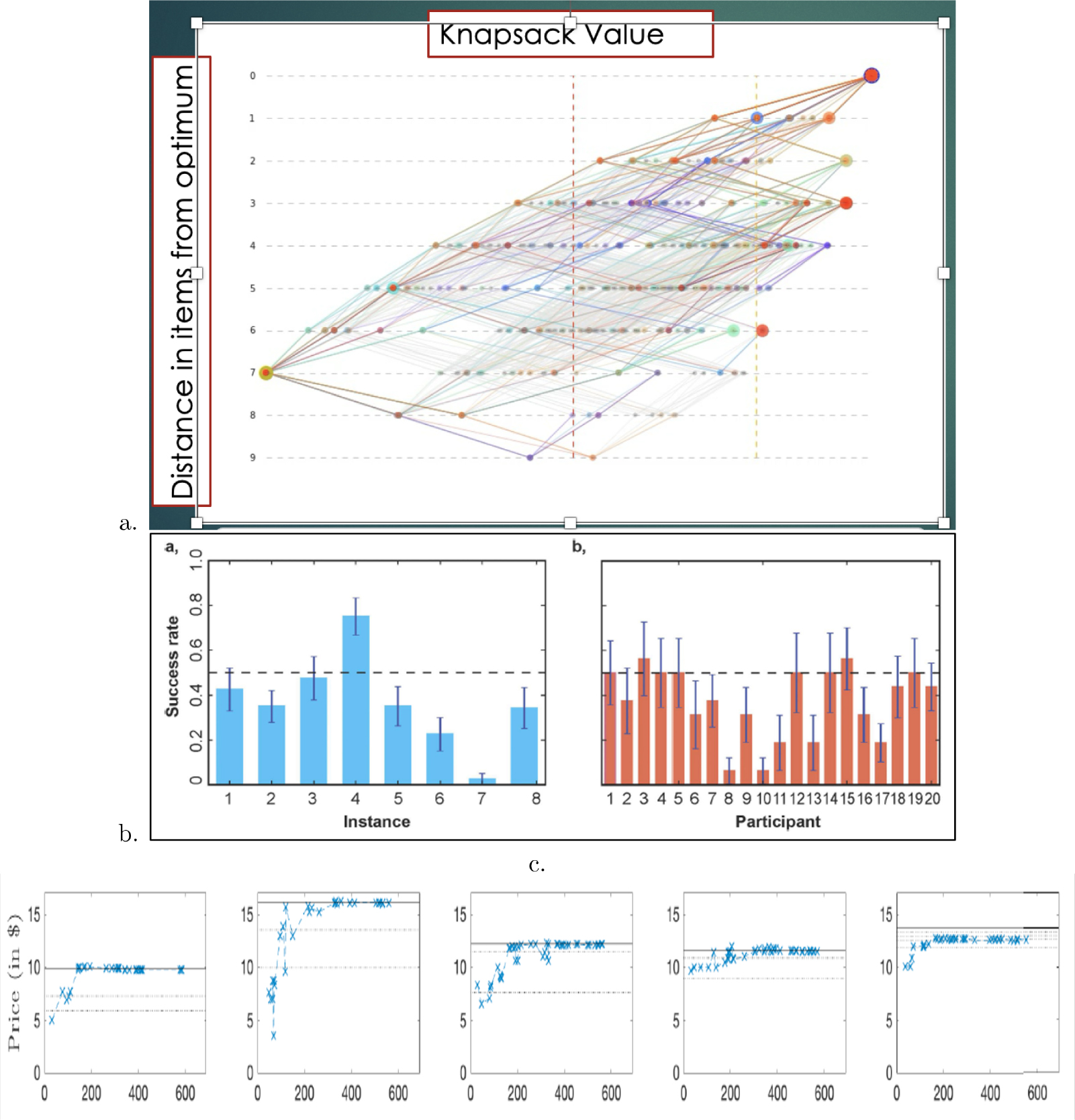
Figure 2. (a) Feasible search paths in item/value space for a knapsack problem (KP) optimization problem with N = 10 items; horizontal: value attained; vertical: distance from the optimal knapsack, in number of items. Participants start with zero items, at which point the value is zero and they are seven items away from the optimum. Each participant-trial (40 in total) is depicted with a different color; large dots indicate final positions. More than 40% of feasible paths are colored, suggesting that search approaches were extremely heterogeneous. (b) Performance, per instance (a) and per participant (b); performance is measured as the fraction of instances where the optimum was found. (a) and (b) reproduced from Murawski and Bossaerts (2016). Evolution of trade prices in a market for a security that paid the true optimal value of a KP optimization instance; five instances are shown. A solid vertical line depicts the optimal value; dotted lines denote the second- and third-best solution values, and for the rightmost instance (the most difficult one; see section 6 on how to measure instance difficulty), up to the fifth best solution. Reproduced from Bossaerts et al. (2024).
(a) Feasible search paths in item/value space for a knapsack problem (KP) optimization problem with N = 10 items; horizontal: value attained; vertical: distance from the optimal knapsack, in number of items. Participants start with zero items, at which point the value is zero and they are seven items away from the optimum. Each participant-trial (40 in total) is depicted with a different color; large dots indicate final positions. More than 40% of feasible paths are colored, suggesting that search approaches were extremely heterogeneous. (b) Performance, per instance (a) and per participant (b); performance is measured as the fraction of instances where the optimum was found. (a) and (b) reproduced from Murawski and Bossaerts (2016). Evolution of trade prices in a market for a security that paid the true optimal value of a KP optimization instance; five instances are shown. A solid vertical line depicts the optimal value; dotted lines denote the second- and third-best solution values, and for the rightmost instance (the most difficult one; see section 6 on how to measure instance difficulty), up to the fifth best solution. Reproduced from Bossaerts et al. (2024).
This does not mean that humans randomly try a solution by picking, in the KP, items at random until the knapsack hits capacity, retrying another random choice while keeping track of the running maximum value. Participants in Murawski and Bossaerts (2016) performed significantly and sizably better compared to random search when random search was allowed the same number of full knapsacks as participants had tried. Figure 2(b) shows that participants’ success rates ranged between 5% and 55%; a random search would have produced a success rate of only 10% (standard deviation: 5%). Note also that success rates varied by instance. In one case, the success rate was only 1/40 (the participant who found the solution in that instance did not discover it again after trying it a second time). Random search would not have produced this effect.
Participants were not compensated based on whether they found the true maximum but on how close their estimate of the maximal value of the knapsack was to the true one. Participants attained, on average, values equal to 97.4% of the optimal value. Random trial and error would have produced a lower average, of 85.3% (p, one-sample t-test). Paradoxically, value estimates became better as effort increased, where effort is measured either as time spent on the attempt (4 minutes maximum) or length of the search path (number of additions/deletions of items in the knapsack). Search continued well beyond the point that the estimated values increased, rejecting the idea that participants stopped when they reached a certain value; they appear not even to be “satisficing” (Caplin et al., 2011; Simon, 1955).
These findings illustrate not only that search is heterogeneous but also that humans rarely optimize. The hypothesis that humans optimize—or act “as if” optimizing—permeates virtually all of economics, including behavioral economics, where maximization is done over a nonconventional utility function such as prospect theory. Recently, attention allocation problems have been of great interest in behavioral economics. There, too, the central hypothesis is that attention allocation is optimal. The assumption of full optimization, whether of budgets or attention, is questionable since it requires agents to solve an NP-hard problem. See Bossaerts et al. (2019) or Gilboa et al. (2021) for further discussion.
Heterogeneity should lead the hypothesis that performance can be dramatically increased by allowing participants to communicate. Various experiments have been conducted where markets are used as a means of communication. The results are compared, for example, with a prize system, where the first person to find the solution walks away with all the compensation that is given to agents as a group; see Meloso et al. (2009). The bottom line is that certain market designs are very effective in spreading knowledge among participants. Successful market designs are discussed in Bossaerts et al. (2024). The market becomes an “oracle” that communicates crucial pieces of information that help participants closer to the best choice.
In many respects, the observations are contrary to those known from experiments in which participants receive free, value-relevant “signals” in probabilistic tasks and in which prices are supposed to average those signals and disseminate the average to all participants. “Bubbles” (overpricing) and “mirages” (markets bet on the wrong outcome) emerge routinely (Camerer and Weigelt, 1991; Corgnet et al., 2023; Page and Siemroth, 2021). When instead values depend on the solution of the KP, the best designs instead lead to prices that always reflect the true knapsack value.
Figure 2(c) provides an example, where the evolution of trade prices for an asset that paid the true optimal solution in five separate instances is shown. Total trading time was 10 minutes (600 seconds) in each instance. Only in one instance did prices not fully converge to the optimal level. This instance was also the most difficult one in terms of a metric of instance difficulty called Sahni-k (to be discussed later). Remarkably, prices never overestimated value, even if participants were allowed to trade at higher prices. That is, a “bubble” never occurred.
The contrast between knowledge dissemination for computationally hard problems and information aggregation in probabilistic tasks reinforces the idea that we started out with—namely, that human attitude toward uncertainty in probabilistic tasks is very different from that in computationally hard tasks. The ambiguity that emerges in the latter is not to be dealt with as some “anomaly,” but it causes systematic behavior that can be harnessed to generate positive outcomes at the group level.
Friedrick Hayek (1945) was the first to point out that traditional economic problems, such as budget allocation or production scheduling tasks, are fundamentally different from information aggregation tasks and that their difficulty must not be underestimated. He hypothesized that markets could play a positive role in the former. He appears to have been right. Interestingly, he wrote all this when the main theoretical concepts and results about computational complexity, to be discussed next, had yet to be derived.
NP-Completeness
So far we have discovered that humans rarely optimize and that the search paths are heterogeneous. To go further, a deeper understanding is needed of the types of combinatorial problems we are dealing with. Hence, we want to dive into the theory of computational complexity. The following is not a comprehensive treatment of the theory of course. Instead, it is a selective reading, with the aim of discovering how a biological computer—the human—deals with complexity, as opposed to an electronic computer, the original object of study in the theory. The digression will be fruitful: it explains in a simple way the paradoxical positive correlation we observed earlier between effort and value attained in the KP: effort indeed increases in difficulty—to be made precise through the theory—and while accuracy (percentage of instances where the solution is found) decreases, high values of more difficult instances happen to be closer together than those of easier instances, so performance, in terms of value attained, increases.
The theory starts with decision problems. These are questions with a definitive answer of “yes” or “no.” For example, can we color vertices of a graph with 4 different hues when there are 27 vertices while no connected vertices should be assigned the same color? Another example is: is it possible to fill a bin with capacity 2 Kg when there are three available items with (value, weight) pairs equal to (1, 1), (2, 1) and (3.75, 2), respectively, so that the value of the bin is at least 3? An instance (instantiation) of a decision problem is the equivalent of an “event” in probability theory, where, once a state is chosen, the event either occurs (the answer is “yes”) or does not (the answer is “no”).
We focus on decision problems where it is easy to check a solution when the answer is affirmative (“yes”). A solution is called a “witness.” “Ease” refers to the fact that the computations needed to check that the witness indeed affirms the instance increases at most as a polynomial in the input size of the instance. In our examples, size is the number of vertices in the graph, or the number of items in the bin. The class of decision problems for which it is easy to verify a witness is referred to as “NP” (nondeterministic polynomial).
Economics focuses on optimization problems while the theory of computational complexity mostly deals with decision problems. This is not an inconvenience. A sequence of instances of a decision problem can become an instance of an optimization problem. In the case of the KP, one can gradually increase the target value that the knapsack is to reach. The optimum (maximum value) is located where the answer to the sequence of instances turns from “yes” into “no.” This then implies that verification of whether an optimum is reached is as difficult as solving the corresponding decision problem.
The class “NP-complete” consists of those decision problems in NP to which all other problems in class NP can be reduced. This means that any other problem can be converted into it in a number of computational steps that are bounded by a polynomial in the input size. Take the graph coloring problem, for instance, with N vertices. This can be converted into a KP of the same size (N items) in a finite number of steps. If the original instance of the graph coloring problem has the answer “yes,” then the corresponding instance of the knapsack problems has as answer of “yes” also. That this can be done may not be obvious.
NP completeness was first proven for the 3-SAT problem, a problem involving logical statements where the question concerns whether they can ever be true (we discuss 3-SAT later). This result, referred to as the Cook-Levin Theorem (Cook, 1983), was proven only in the 1970s, and set off the theoretical analysis that forms the foundation of our investigation of human attitudes toward computational complexity.
Since all NP problems need to be reduced to a candidate NP-complete problem, the class NP-complete contains the most difficult NP problems. The graph coloring problem, KP, and 3-SAT are three examples of members of the class NP-complete. The core, hitherto unanswered question is: how difficult are NP-complete problems?
To answer this question, we need the concept of an algorithm. An algorithm is a sequence of computational steps that eventually, in a finite, albeit perhaps very large, number of steps reaches the correct answer. The steps are deterministic. The question is, is there an algorithm that guarantees that the number of computations needed to solve an NP-complete problem is bounded by a polynomial in the size of the instances N? At the time of writing, the answer is no. That is, for any algorithm tried so far, one can always find a sequence of instances such that the number of computations increases faster than any polynomial. In this sense, NP-complete problems are intractable. This feature is used in cryptography (see, e.g., Arora and Barak, 2009, chapter 9).
Decision problems can be converted into optimization problems, as discussed before. When the original decision problem is NP-complete, the resulting optimization problem is referred to as NP-hard. Importantly, the asymmetry we referred to before does not apply to optimization problems. The determination of whether an optimum has been reached is a problem in the class NP-complete. This contrasts with classical optimization problems in economics, where sufficient smoothness is assumed so that it becomes easy to verify whether an optimum has been reached by calculating first and second derivatives. Software on an electronic computer that solves NP-hard problems can never tell one how much time it needs for a given instance. This is the source of ambiguity in NP-hard problems.
Importantly, here we sketch the situation as of the writing of this paper. One day some clever mathematician could find an algorithm that solves an NP-complete problem in polynomial time. Because all NP-complete problems can be reduced to it, this mathematician will have found an algorithm that solves all NP-complete problems. In short, she will have proven that “P = NP”: all NP problems can be solved in polynomial time (i.e., they all belong in the class “P”). NP-hard problems are not “more difficult.”
A consequence is that a uniformly best algorithm, one that could be used to “nudge” people to become more efficient in search for a solution, does not exist yet. Even for problems of the size we consider here (e.g., KP with 6 to more than 20 items), there is not one. Students of the KP optimization problem are often told to use dynamic programming, but even the brute-force algorithm (which is to list all feasible solutions, sort them, and pick the one that reaches the highest value) is in general far more efficient when the size of the instance is low. Relatedly, Pape et al. (2020) consider the optimization version of the KP. They claim that humans are biased toward solutions that are too small (relative to the optimum). They advocate “nudging” toward larger knapsacks by putting all available items in the solution and asking people to delete the items that they think do not belong until reaching the capacity limit (from above). However, the bias they identify cannot be generic. It is specific to the instances they selected. It may not be present in other sets of instances. Their nudge is ill-advised, since the bias may not apply to the instances that their participants encounter in daily life.
There is a general understanding that there is no uniformly best efficient algorithm (one that solves NP-hard problems in polynomial time). But one needs to appreciate the implications when one day it is found, contrary to expectation. In computer science, interest in NP-hard problems as a class will certainly wane since computer scientists will no longer treat NP-hard problems as somehow “distinct.” But, as we demonstrate, the classification (and related ones) matters to predict human choice and effort (and, as we shall see, nonhuman primate choice as well). That is, the features that allow us to claim that a problem is NP-hard reflect fundamental properties with which to predict human behavior.
Unfortunately, the uncertainty surrounding whether P = NP makes the application of the theory of computational complexity to human behavior extremely delicate and, in my view, easily misunderstood. We do not want to derive hypotheses based on an assumption (“P ≠ NP”) that may prove one day to be wrong. We necessarily will be working with hypotheses that are only loosely but reasonably related to the theory. One obvious hypothesis is whether humans do better on problems in P than on NP-hard problems, or whether they need less effort on them. This is a reasonable hypothesis, because most experts believe that problems in P are easier, but it is only loosely related to the theory, because it is not known whether the belief is true. Our position is that humans distinguish between P and NP-hard problems because they are somehow felt to be distinct, and this allows us to formulate behavioral hypotheses.
We do not compare performance between P and NP-complete problems, instead focusing on the latter only. The class NP-complete is constructed from algorithms that find the correct solution. But, as we found out in the previous section, humans often do not—or do not care to—work all the way to the correct solution. As such, in principle the theory again cannot shed light on human behavior since the algorithms of the theory always find the correct solution (by definition). Still, it could be that there are common features in all NP-complete problems that could be used to predict effort and performance. And indeed there are.
One of those features is the existence of a “phase transition:” a region in the space of instances where all the difficult instances are, regardless of the algorithm used. Such a region has been found for a number of NP-complete problems, such as TSP (Gent and Walsh, 1996), 3-SAT (Monasson et al., 1999), and KP (Yadav et al., 2020). The region provides a boundary between instances for which the answer is predominantly “yes” (i.e., solvable [the region of underconstrained instances]) and instances for which the answer is predominantly no (i.e., unsolvable [the region of overconstrained instances]). Instances in the phase transition tend to be difficult; outside, they are easy.
The existence of a phase transition in NP-complete problems allows us to recognize difficulty ex ante. This suggests the following behavioral predictions: (i) chances of humans to find the correct solution are lowest for instances in the phase transition, and (ii) effort expended (e.g., time on task) is highest in the phase transition. Again, these predictions do not follow as an immediate consequence of the theory since the theory focuses on algorithms that guarantee the correct solution at the end of computations. The link between theory and behavioral predictions is loose, as emphasized before. But, as we shall see, the predictions work.
Franco et al. (2022) report results from an experiment where instances of 3-SAT, TSP, and KP were selected from in and outside the phase transition, stratified by solvability (whether the decision problem instance has “yes” as its answer). See figure 3(a) for a visual representation of the three problems. As it turns out, accuracy (the chance of finding the correct answer) is indeed determined in large part by whether the instance is inside or outside the phase transition. See figure 3(b). The situation is more complex as far as effort (time on task) is concerned [same figure section, panel (b)]. Effort is indeed highest on average in the phase transition, but paradoxically, it is also high outside the phase transition when instances are unsolvable.
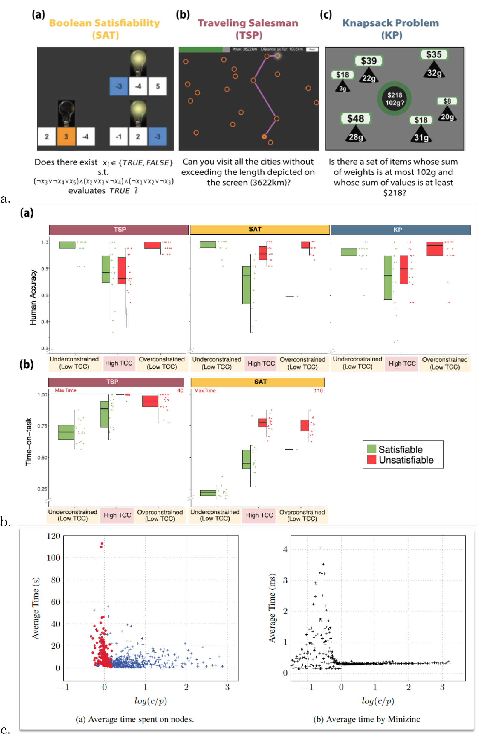
Figure 3. (a) Visual representation of instances of three NP-complete decision problems: 3-SAT (left), traveling salesperson problem (TSP; middle), and knapsack problem (KP; right). (b) Boxplots of human performance (a) and effort (b) in the three problems (effort for the KP is not shown since it was not self-paced); instances are stratified in terms of typical case complexity (TCC; whether in or outside the phase transition) and solvability (“satisfiability:” red indicates that the correct answer was “yes;” otherwise green color is used). (a) and (b) reproduced from Franco et al. (2022). (c) Time needed to increase value in the KP optimization problem or declare that an optimum has been reached, as a function of the log-ratio of normalized capacity c and normalized values p, for humans (a) and machines (electronic computer) (b). Humans solved instances of 10 items, not always correctly; a computer program (MiniZinc) solved instances of 50 items, always correctly. A phase transition is discernible, where the log-ratio is close to and below zero. Reproduced from Yadav et al. (2020).
(a) Visual representation of instances of three NP-complete decision problems: 3-SAT (left), traveling salesperson problem (TSP; middle), and knapsack problem (KP; right). (b) Boxplots of human performance (a) and effort (b) in the three problems (effort for the KP is not shown since it was not self-paced); instances are stratified in terms of typical case complexity (TCC; whether in or outside the phase transition) and solvability (“satisfiability:” red indicates that the correct answer was “yes;” otherwise green color is used). (a) and (b) reproduced from Franco et al. (2022). (c) Time needed to increase value in the KP optimization problem or declare that an optimum has been reached, as a function of the log-ratio of normalized capacity c and normalized values p, for humans (a) and machines (electronic computer) (b). Humans solved instances of 10 items, not always correctly; a computer program (MiniZinc) solved instances of 50 items, always correctly. A phase transition is discernible, where the log-ratio is close to and below zero. Reproduced from Yadav et al. (2020).
The last finding is paradoxical because one can determine ex ante whether an instance is overconstrained and hence whether it is predominantly unsolvable. Then again, it was not until recently that computer scientists discovered the location of the phase transitions (see previous citations), and hence phase transitions were unlikely to be known to participants. The tendency to spend more effort on unsolvable instances may be related to the asymmetric uncertainty typical of NP-complete problems: once a witness for an affirmative answer is found, one is sure—barring arithmetic mistakes—that while as long as a witness has not been found, it remains unclear whether the instance is truly unsolvable unless one has tried out all possibilities (or used an algorithm that guarantees the correct solution). Thus, participants may have continued the search until cognitive exhaustion, at which point they stopped searching and declared the instance unsolvable, mainly correctly.
This then suggests that participants may not even have allocated effort ex ante. Participants may have started solving an instance with an amount of effort irrespective of the ex ante recognizable difficulty of the instance at hand. For solvable instances, they then found that the answer was affirmative and stopped. The time to stopping was shorter for underconstrained instances since they were easier, and a bit longer for solvable instances in the phase transition. If the instance was unsolvable, participants continued search until a particular point that was independent of whether the instance was inside or outside the phase transition, eventually declaring the instance unsolvable. As a result, since the vast majority of instances outside the phase transition are indeed unsolvable, their accuracy was much higher than for instances inside the phase transition.
So perhaps humans do not allocate effort ex ante? This possibility seems to contradict the core idea behind the theory of cognitive effort allocation (including allocation of attention). There, the decision-maker must first examine the features of the problem at hand to determine how much effort is required given constraints on (neurobiological) resources. This idea has become known as the “resource rationality hypothesis” (Lieder and Griffiths, 2020). Consistent with the lack of ex ante effort allocation, we later document that, early on in the search for a solution, brain signals do not correlate with ex ante markers of difficulty and solvability.
Figure 3(b)[b] does not display results for KP since time allowed was too short (20 seconds instead of 40 for TSP and 110 for 3-SAT) to meaningfully dissociate effort as a function of difficulty and solvability. In a KP experiment with far more lenient decision times, Yadav et al. (2020) report that the time spent in the phase transition is the longest. See figure 3(c).
The time spent by an electronic computer using standard solution protocol shows a strikingly similar pattern to that of humans; see figure 3(c). Interestingly, the left tail in time spent shows that electronic computers too ignore the fact that overconstrained instances (which are in the left tail in the plot) are predominantly unsolvable. Like humans, the electronic computer does not appear to allocate effort ex ante. In the case of the electronic computer, this is because it does not guess. It uses an algorithm that will for sure give the correct answer and will work at it until it finds it. Effort required is longer for all unsolvable instances, though a bit less the more constrained the instance becomes (beyond the phase transition).
A Digression on “Encoding”
The presentation of instances of computationally complex problems is not straightforward. By their very nature, a lot of information has to be displayed at once. Take, for instance, the KP decision problem. If there are N items, 2 N + 2 numbers are involved: the values and weights of each of the items, the capacity of the knapsack, and the target value. In TSP with N nodes, up to distance numbers must be considered. With a typical working memory of 5 to 10 slots, humans cannot possibly simultaneously encode all those numbers even for KP instances as small as N = 4 or TSP instances with N = 5 nodes.
As such, there is an issue of encoding—that is, the mental (neural) representation of the data that defines the instance of the problem. One can focus attention on algorithms that use memory parsimoniously, but none of the theoretical analysis so far does, and none of the theoretical analysis to follow will. That is, the computers behind the theory we appeal to here (so-called Turing machines) are allowed to use as much memory as they like. The algorithms are not “space constrained.” Extensions to space-constrained algorithms is an important topic of further investigation and one that has only recently caught the attention of economists (e.g., Sanjurjo, 2015, 2023).
Meanwhile, we must be aware of the amount of data that humans have to process. Biases in decision-making can emerge for the simple reason that participants only consider a small fraction of the inputs. A possible approach is to represent the problem instance in terms of a summary approximation, using a parsimonious “reference model” of the problem that ensures that as little information from the true instance is lost before proceeding to the solution stage.
The idea that a reference encoding model is used in decoding first emerged in computational neuroscience as a result of the discovery of the nature of limitations in neural processing of sensory stimuli (signals), such as visual or auditory cues. It became apparent that the brain was using simplified reference models—simplified to make subsequent computations feasible given the neurobiological constraints—suitably adapted to minimize loss of information (Attneave, 1954; Barlow, 1961).
To gauge the importance of the problem of encoding, let us consider simple probabilistic tasks, such as choosing from a deck of 10 cards in a card game. It is possible to represent the information in as intuitive a way as possible, to the point that neural signals of the game’s stochastic properties (e.g., expected rewards; reward risk) emerge in the brain in a fraction of a second (see, e.g., Preuschoff et al., 2008). However, in most experiments, probabilistic tasks tend instead to be represented more formally, in a “descriptive” way. For example, the participant may be asked: “Imagine a lottery in which one can earn $1.50 with chance 0.3, lose $0.50 with chance 0.4, and otherwise earn nothing.” It is not easy to encode the information in this question.
Not surprisingly, the need for encoding has recently been shown to cause well-known cognitive biases such as probability weighting. This means that cognitive biases emerge not only because humans adapt simple heuristics—the traditional view, according to Tversky and Kahneman (1974)—but also because of the need to encode, from the available information, what the problem is that the participant has to decide on. The evidence so far demonstrates that, as with perceptual tasks, the brain uses parsimonious reference models of the probabilistic problem at hand, adapted to maximize mutual information between the true problem and its mental (neural) representation in terms of the reference model (Azeredo da Silveira & Woodford, 2019; Polanía et al., 2019; Vieider, 2024; Yamada et al., 2018).
If encoding is such a big issue with simple probabilistic tasks, one can imagine that it affects decision-making even more in computationally complex tasks. This is not a problem when, as in the experiment behind figure 2(b), we compared same-sized instances of a single problem. But it becomes problematic when comparing instances with differing sizes, or when comparing instances across problems.
For example, in figure 3(a), the sizes of the problems are: N = 5 (3-SAT), N = 20 (TSP), and N = 6 (KP). The sizes are vastly different. But the amount of information to be encoded is not a fixed function of the input sizes. While 3-SAT instances are the smallest, far more information has to be absorbed, namely the composition of the three clauses. The size of the KP instances is also small, certainly compared to TSP, but then again, each item in KP comes with two data points, value and weight, while each edge in TSP comes with only one number (the distance). In the case of figure 3(a), the researchers ended up choosing sizes to make the encoding difficulty comparable, based on the conjecture that comparability is obtained if performance across the problems was similar.
It may be surprising that the theory (of computational complexity) would not take the complexity of encoding into account. After all, even a Turing machine has to read the input. The theory calculates the input size in a disciplined way, unlike what we have been doing so far. When measuring the size of, say, the KP optimization problem, we counted only the number of items. This is not correct. The input string that the Turing machine has to encode consists of all weights and values of all items plus the capacity of the knapsack. This amounts to 2 N + 1 numbers if N is the number of items. When represented in binary format, the total length of the string that represents these 2 N + 1 numbers is the true size of the input. Likewise, one may have thought that the size of the TSP equals the number of vertices of the graph, N. The input size equals N(N − 1) numbers in binary format provided all vertices are connected, since each edge has a distance number. If not all vertices are connected, then the input size is lower. In general, the input size is directly related to the number of edges instead of the number of vertices.
In conclusion, one has to be careful in measuring the true size of a problem instance. It is the length of the string of binary digits that a Turing machine needs to read to encode all the relevant data for a problem instance. When the true length becomes excessive for humans, the foregoing discussion becomes relevant. So far, we do not know when this will happen.
Approximation Complexity
Since humans apparently do not strive to always find the correct solution, maybe we should not pay attention to a theory that focuses on algorithms that guarantee the solution but instead turn to approximation algorithms. These are algorithms that use an internal clock (based on evidence gathered) to decide to stop, without guaranteeing that the answer provided is correct.
We focus on optimization problems and study only approximation algorithms that are “good” in the sense that they guarantee minimum performance in terms of value attained relative to optimal value. The theory has provided a classification of problems into “easy,” “difficult,” and “impossible to approximate.”
An approximation algorithm can be thought of as a heuristic. The theory of approximation complexity will help us answer an important question that should have been posed in the context of the heuristics and biases program started by Tversky and Kahneman (1974): Are the heuristics humans deploy adapted to the difficulty at hand? Gigerenzer and Selten (2002) claim that heuristics are optimal for some problem instance, while for others, presumably less frequently visited ones, heuristics can be arbitrarily bad. Here, we take the view that the heuristic has to have minimal performance regardless of the problem instance.
As we study minimization problems, let R(x, w) denote the ratio of value w attained by an approximation algorithm and the correct minimal value w* given the vector of inputs x,
We want good algorithms, which we mean that, for all x,
given a critical value r, while time to compute the solution remains bounded by a polynomial in the size of the problem. If such an algorithm exists for some r, then the problem is approximable. It is said to be in the class APX. For example, in KP, replacing the criterion with that of minimizing minus the weighted sum of values of items in the knapsack, the greedy algorithm discussed before has r = 2. Hence, KP ∈ (is in the class) APX.
An example of a problem for which such an r does not exist is the non-Euclidean traveling salesperson problem (non-ETSP). In a TSP, the goal is to find the shortest path that visits all nodes in a network without repeating any visit. In the non-ETSP, network distances are random and hence violate Euclidean distances because, for instance, the shortest path between A and B runs through a third node C. We can think of the randomness in this random TSP (RTSP) as the result of random congestion. In RTSP, there is no r so that (1) holds. RTSP is said to belong to the class NPO.
An NP-hard minimization problem is in the class PTAS if there exists an algorithm that, fixing r, computes a solution with value w in time bounded by a polynomial in the size of the instances N (size of x) and the solutions have . We call members of PTAS polynomial-time approximable. An example is the TSP when the network is constructed in Euclidean space. We refer to this as the Euclidean TSP (ETSP).
When solution times are bounded by a polynomial in both N and then the minimization problem belongs in FPTAS and is said to be fully polynomial-time approximable. Both KP (when converted to a minimization problem) and the weighted cost shortest path problem (WCSPP) are members of FPTAS. In the WCSPP, one is to find the shortest path between two points in a Euclidean network when feasible transitions between nodes come not only with a distance but also with a cost, and the total cost has to remain within a bound.
The existence of a nontrivial class of nonapproximable problems implies that approximating solutions well can be as difficult as finding the solution itself. The statement remains true even if one day it is proven that P = NP. But the theory does not imply that somehow problems in FPTAS are easiest. They are only thought to be easiest, as of this writing. This is annoying because the theory does not immediately link to a precise prediction about human performance.
However, we can formulate a hypothesis about human performance that is more loosely related to the classification. The one that springs to mind is that, fixing N (the size of the problem), performance is best in WCSPP and worst in RTSP. We measure performance as R(x, w). The hypothesis is not based on the premise that WCSPP is easiest and RTSP most difficult, because that is not what the theory says. The hypothesis is based on the belief that (i) there are features of those problems that somehow put them in separate classes because of how humans at present think they can best solve them and (ii) these features can be used to predict human performance.
Since RTSP, ETSP, and WCSPP can conveniently be depicted with the same interface (see figure 4(a)), we could test our hypothesis without participants being made aware that we are recording performance (and effort) on problems across three different complexity classes.
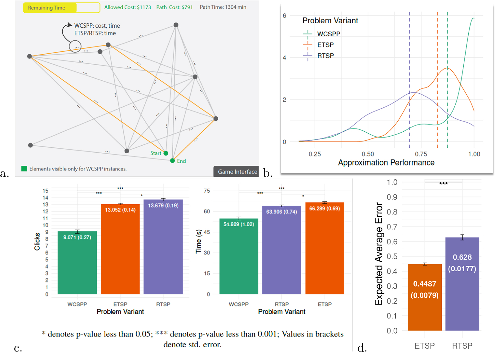
Figure 4. (a) Three graph problems: random traveling salesperson problem (RTSP), where the shortest feasible path is to be found connecting all nodes without visiting any node twice; Euclidean traveling salesperson problem (ETSP), like RTSP, but where distances (indicated with ⋯) satisfy Euclidean restrictions; and weighted cost shortest path problem (WCSPP), where the path with the shortest distance has to be found between a Start and End point while costs from feasible transits remain within a limit. (b) Kernel densities of human performance [R(x, w)] in the three problems. (c) Effort in the three problems in terms of the number of mouse clicks (left) or time (right). (d) Expected average error [] from randomly choosing feasible paths is higher in RTSP than in ETSP despite an equal number of feasible paths. All panels reproduced from Yadav et al. (2024).
(a) Three graph problems: random traveling salesperson problem (RTSP), where the shortest feasible path is to be found connecting all nodes without visiting any node twice; Euclidean traveling salesperson problem (ETSP), like RTSP, but where distances (indicated with ⋯) satisfy Euclidean restrictions; and weighted cost shortest path problem (WCSPP), where the path with the shortest distance has to be found between a Start and End point while costs from feasible transits remain within a limit. (b) Kernel densities of human performance [R(x, w)] in the three problems. (c) Effort in the three problems in terms of the number of mouse clicks (left) or time (right). (d) Expected average error [1−1/ R(x,w)] from randomly choosing feasible paths is higher in RTSP than in ETSP despite an equal number of feasible paths. All panels reproduced from Yadav et al. (2024).
In view of our discussion in the previous section, we need to check whether the input sizes of the three problems (WCSPP, ETSP, and RTSP) are comparable. We previously computed the true input size of TSP as the number of edges, not the number of vertices. Since each edge contains two numbers, distance and cost, and there is a capacity constraint, the input size of WCSPP equals twice the number of edges plus 1. To make the input sizes of the three problems comparable, we therefore have to make sure that about twice as many edges are included in the TSP problems (ETSP and RTSP) compared to WCSPP. Here, we discuss human effort and performance for networks with 45 edges connecting 10 vertices in the ETSP and RTSP. We then compare the results for the WCSPP when the same 10 vertices are displayed but connected by only 23 edges. Confirming our hypothesis, Yadav et al. (2024) report that participants achieve better performance [measured as R(x, w)] in WCSPP, followed by ETSP, and lastly RTSP. See figure 4(b). Not only is this true on average (dashed lines), but the entire distribution shifts to the left as one moves from WCSPP to ETSP and RTSP. Importantly, the decrease in performance occurs for virtually all of the 24 participants individually.
A further hypothesis one could formulate in view of the theory is that productivity (increase in performance) per unit of effort is highest in WCSPP and lowest in RTSP. Effort can be measured as time spent (in seconds) or number of mouse clicks in the computer interface used in the experiment. Again, this is borne out in the data. See figure 4(c).
In terms of both performance and productivity, it appears that human effort and performance align well with the theoretical classification of problems in terms of approximation complexity. Performance and productivity are worst for instances of a member of NPO and best for a member of FPTAS. Clearly, these classes capture something real. That is, the features of the problems in these classes must somehow be different, and these differences matter in the prediction of human behavior. Even if one day it is shown that P = NP and the classification becomes computationally inconsequential, they should still be behaviorally relevant.
How would we discover these features? Let us consider ETSP and RTSP, which are sufficiently similar that comparisons become meaningful because they have exactly the same number of feasible paths (in the experiment: 181,440). Moreover, each path from beginning to end that does not visit a node twice is a feasible solution for both problems. Each feasible path can be considered the suggested solution of some algorithm. Now remember that human search paths in NP-hard problems appear to be very heterogeneous. In principle, humans could have chosen any feasible path as a solution. We can therefore simulate human behavior by uniformly drawing feasible paths and determine to what extent average performance is higher in ETSP than in RTSP. The sampling is biased relative to human behavior since humans do not pick feasible solutions with uniform probability (humans perform significantly better). But uniform drawing constitutes a neutral way to compare the two problems: there is no prejudice about which feasible paths are “better,” and the same amount of effort is applied.
Random drawing thereby could prove that there are differences in features between the two problems that explain why humans perform better in ETSP than in RTSP. This is exactly what happens. As shown in figure 4(d), the expected average error [measured as ] is significantly and sizeably higher in RTSP, in line with the lower human performance.
Algorithm-Dependent Metrics of Difficulty
Among the many algorithms that have been proposed to solve the KP optimization problem, the greedy algorithm stands out, not only because of its simplicity but also because it is the right algorithm to use when items are infinitely divisible. Hence, the greedy algorithm provides a bridge for economists to understand how indivisibilities affect a core economic problem: that of allocating a budget among scarce goods. The greedy algorithm also stands out because, if it correctly finds the optimum, then humans evidently tend to use it to construct their first estimate of the optimal knapsack; see Murawski and Bossaerts (2016).
The greedy algorithm is also the starting point of a number of algorithms that find the solution, such as the Sahni-Horowitz algorithm (Sahni, 1975). The idea is to use the greedy algorithm to come up with a first estimate of the optimal solution, then selectively replace items to improve the estimate. This can be used to construct a metric of difficulty that has proven to be useful in predicting human performance and effort in the KP optimization task, which we refer to as “Sahni-k” (Meloso et al., 2009). When the greedy algorithm produces the optimal solution, we say that the instance has Sahni-k=0. When an item must already be in the knapsack before the greedy algorithm can be used to find the solution, then Sahni-k=1. When two items must be in the knapsack before the greedy algorithm finds the solution, then Sahni-k=2, and so on. Difficulty increases in Sahni-k.
Figure 5(a) demonstrates that Sahni-k is effective in predicting human performance (percentage correct answers) in one of the first experiments that tested the relationship with instances of sizes . When collating 4,705 attempts from multiple experiments with instances of the same sizes, the regression slope of performance on Sahni-k equals –0.12. The slope is highly significant: . Increasing Sahni-k one notch decreases the value attained (as a percentage of the optimal value) as much as increasing the number of available items by five. There is significant interaction, though: increasing the number of items by one offsets the negative impact of a decrease in Sahni-k by 1 point.
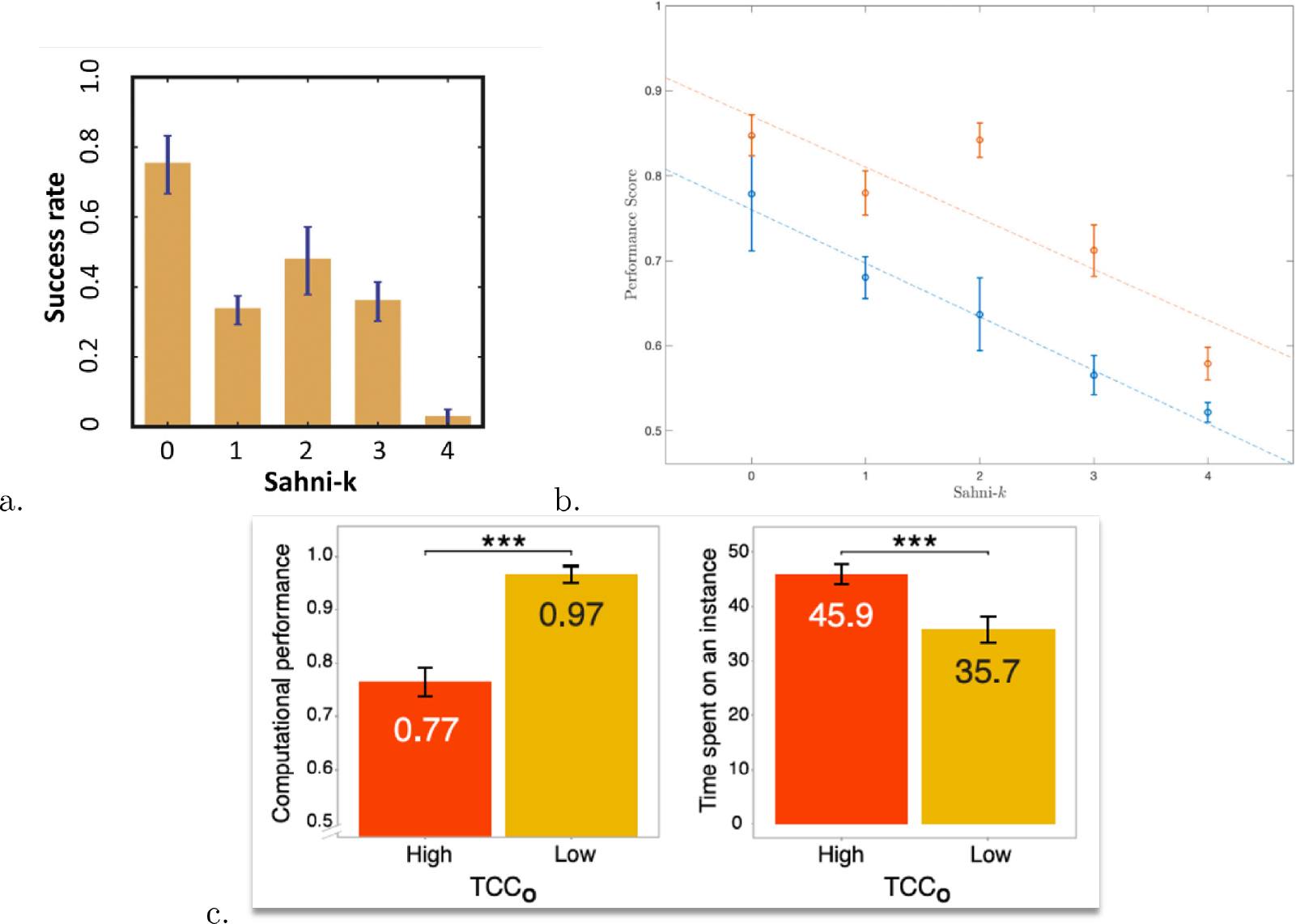
Figure 5. (a) Individual performance (percentage instances solved correctly) in the knapsack problem (KP) optimization problem with items as a function of Sahni-k; 20 participants, 16 instances. Reproduced from Murawski and Bossaerts (2016). (b) Performance of an algorithm based on market prices of binary options that pay 1 if the corresponding item is in the optimal solution and 0 otherwise (blue), against performance of individual traders in the marketplace (red), as a function of Sahni-k. Humans do significantly better than individuals on average; between 18 and 20 participants per marketplace. Reproduced from Bossaerts et al. (2024). (c) Individuals’ performance and effort in KP (optimization), as a function of typical case complexity; 20 participants, 18 instances of N = 6 items each. Reproduced from Franco et al. (2021).
(a) Individual performance (percentage instances solved correctly) in the knapsack problem (KP) optimization problem with N=10,12 items as a function of Sahni-k; 20 participants, 16 instances. Reproduced from Murawski and Bossaerts (2016). (b) Performance of an algorithm based on market prices of binary options that pay 1 if the corresponding item is in the optimal solution and 0 otherwise (blue), against performance of individual traders in the marketplace (red), as a function of Sahni-k. Humans do significantly better than individuals on average; between 18 and 20 participants per marketplace. Reproduced from Bossaerts et al. (2024). (c) Individuals’ performance and effort in KP (optimization), as a function of typical case complexity; 20 participants, 18 instances of N = 6 items each. Reproduced from Franco et al. (2021).
The relation with Sahni-k also holds for choices made by nonhuman primates. With the subset-sum problem (a variation of the KP optimization problem in which items only feature rewards and items have to be added to a basket to get as close as possible to a target reward without exceeding this reward), Hong and Stauffer (2023) report that the performance of two monkeys decreases significantly as a function of Sahni-k.
The relation with Sahni-k holds for market prices as well. For example, consider prices of binary options associated with the items of a KP optimization problem: one option pays a reward when the corresponding item is in the optimal solution and zero otherwise. Meloso et al. (2009) showed that the final prices in an anonymous continuous open-book market could be used to formulate a simple algorithm with which to obtain suggested solutions of the KP with 10 or 12 items. The performance of this algorithm decreased in Sahni-k. The result was replicated more recently in Bossaerts et al. (2024; see figure 5(b)) and extended to a market where only one security was traded, and this security paid the value of the optimal knapsack.
Unlike the phase transition for decision problems, Sahni-k cannot be used as an ex ante metric of difficulty, because it cannot be computed without knowing the optimal solution. It is possible to adapt the phase transition for decision problems and define an alternative to Sahni-k for optimization problems. Franco et al. (2021) show how the location of the decision problem instance corresponding to the optimal value in the optimization version can be used to predict human performance and effort. The metric, known as typical case complexity (TCC), measures how far the decision problem instance is from the phase transition when the target value in this decision problem is set equal to the optimal value. In Franco et al. (2021), it is shown that both Sahni-k and TCC predict performance and effort. See figure 5(c) for the relationship between TCC and performance and effort. The effect of Sahni-k on effort disappeared when competing with TCC. This may be obtained merely because instances were not selected to maximize power with respect to Sahni-k but only with respect to TCC.
Like Sahni-k, TCC is not an ex ante metric of difficulty: one has to know the optimal value of the knapsack to compute TCC. As such, the relation between effort and Sahni-k and/or TCC may be purely spurious because easier instances are solved more quickly, which means that difficulty spent predicts effort ex post.
In markets, there is emerging evidence that the bid-ask spread (the difference between the best offer to buy and the best offer to sell) signals Sahni-k as early as 30 seconds within a trial, even for knapsack instances of 10 to 12 items (Bossaerts et al., 2024). Again, there could be a mechanistic explanation: it could merely be the effect of order submission by the few participants who find the solution very quickly, which we expect to be faster when difficulty is lower.
Neural Foundations
One way to investigate whether effort allocation correlates with difficulty metrics such as location relative to the phase transition or solvability is to track neural activation. In the absence of early neural signals correlating with such metrics, it is doubtful that effort allocation could be based on them. Of course, the method used may lack power. But studies of probabilistic tasks such as multiarmed bandit choice have demonstrated convincingly that neural signals related to mathematical aspects of the problem at hand can be tracked early on in a trial, even by means of 3-Tesla functional magnetic resonance imaging (fMRI); see, for example, Payzan-LeNestour et al. (2013). Here, we study brain activation tracked by means of 7-Tesla fMRI while participants solved instances of the KP decision problem.
Figure 6 is taken from Franco et al. (2024). Panel (b) shows time courses of activation in three regions of interest in the human brain. The regions were chosen because of their proven relevance in decision-making under uncertainty: anterior insula, engaged in uncertainty tracking; dorsal anterior cingulate cortex, involved in cognitive control; and angular gyrus (AG)/intraparietal sulcus(IPS), active when computations or logical deduction are needed. For localization of those regions, see figure 6(a). Time courses in figure 6(b) are stratified by (i) difficulty as measured by TCC (“complexity”) and (ii) solvability (“satisfiability”). The figure shows that separation along complexity and solvability is obtained convincingly only in the later stages of the trial, at 20 seconds or later, and close to the point at which the participant had to decide whether the decision instance was solvable. The significant separation of neural time courses in later stages suggests that we should also have been able to separate in earlier stages, but we were not. All instances featured six items and were chosen to maximize spread across the two dimensions (complexity; solvability).
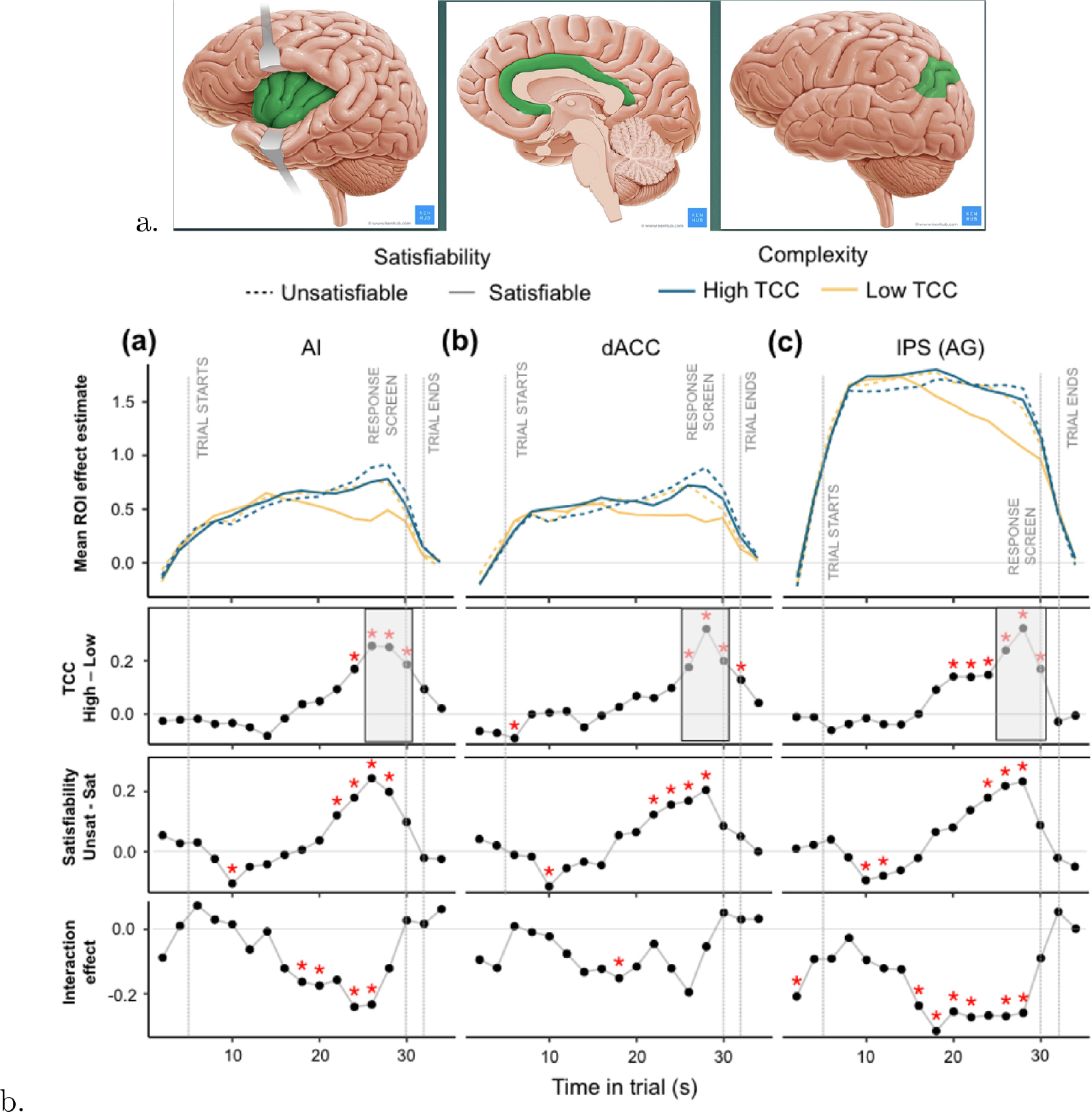
Figure 6. (a) Brain regions of interest (ROI): insula [only anterior part (AI) is of interest]; cingulate cortex [only dorsal–upper–anterior part (dACC) is of interest]; angular gyrus (AG)/intraparietal sulcus (IPS). (b) Time courses and differences relative to start time of a trial but adjusted for a 5 second fMRI signal delay; average across participant-trials extracted using random-effects general linear modeling and stratified by solvability (satisfiability) and typical case complexity (TCC). High TCC = target value is in the phase transition; low TCC = target value is outside phase transition, and hence, the instance is either underconstrained (and hence solvable) or overconstrained (and hence unsolvable). Red asterisks indicate significant differences at . Significance levels in grey-colored epochs in the TCC plots are suggestive only because they do not correct for the fact that the ROIs were extracted from whole-brain corrected neural activation difference for the shown contrast (TCC) during the epoch indicated. All panels reproduced from Franco et al. (2024).
(a) Brain regions of interest (ROI): insula [only anterior part (AI) is of interest]; cingulate cortex [only dorsal–upper–anterior part (dACC) is of interest]; angular gyrus (AG)/intraparietal sulcus (IPS). (b) Time courses and differences relative to start time of a trial but adjusted for a 5 second fMRI signal delay; average across participant-trials extracted using random-effects general linear modeling and stratified by solvability (satisfiability) and typical case complexity (TCC). High TCC = target value is in the phase transition; low TCC = target value is outside phase transition, and hence, the instance is either underconstrained (and hence solvable) or overconstrained (and hence unsolvable). Red asterisks indicate significant differences at p=0.05. Significance levels in grey-colored epochs in the TCC plots are suggestive only because they do not correct for the fact that the ROIs were extracted from whole-brain corrected neural activation difference for the shown contrast (TCC) during the epoch indicated. All panels reproduced from Franco et al. (2024).
After 20 seconds, participants generally found the correct solution to solvable (“satisfiable”) instances of low complexity (i.e., those outside the phase transition). In principle, participants should also have been able to quickly identify the unsolvable (infeasible) low-complexity instances (low TCC) since they tend to be overconstrained. Yet we know that humans do not do so. Instead, as discussed before, they tend to continue searching (see figure 3(b)). This causes an interaction effect between complexity (TCC) and satisfiability later in the trial.
As with behavior, the time courses of neural activity thus point to the possibility that cognitive effort allocation is not ex ante but instead correlates with difficulty metrics purely because some instances can be solved almost immediately, while others will take more time, even when it should be obvious from the beginning that they may not be solvable at all. However, neither the behavioral nor the neural evidence is conclusive proof of this possibility. More research is needed.
Figure 4 in Franco et al. (2021; not reported here) suggests that humans stop searching in the KP optimization problem when the time needed to update the choice reaches a certain limit: regardless of the difficulty of the instance at hand (which was measured as TCC), the search stopped when it took participants 20 seconds to find a better choice. Choice revisions were identified as mouse clicks that altered the composition of the chosen knapsack. The 20 seconds should not be considered a golden rule; presumably the duration is modulated by the total time available to make a decision (and the opportunity cost of time). In Franco et al. (2021), 60 seconds were allowed, while in Franco et al. (2024), only 25 seconds were allotted (the choice had to be indicated in the epoch between seconds 25 and 28).
An alternative way to investigate the nature of the effort spent on a computationally complex task is to administer drugs such as methylphenidate, dextro-amphetamine, or modafinil. These are so-called smart drugs because they are widely used among higher education students or by finance and medical professionals to boost their mental productivity and endurance (Bowman et al., 2020).
In a within-subject double-blind clinical trial with 40 participants, Bowman et al. (2023) showed that, while accuracy (percentage of instances solved correctly) decreased insignificantly (), value attained in KP deteriorated significantly under smart drugs (). Participants were asked to solve eight instances and were granted two attempts at each. The reduction in performance emerged despite a significant increase in effort for methylphenidate and dextro-amphetamine (time spent; ), analogous to the increase in exploration in the bandit problem under methylphenidate. As a result, productivity, measured as an improvement in value per choice review, decreased significantly; see figure 7(a).
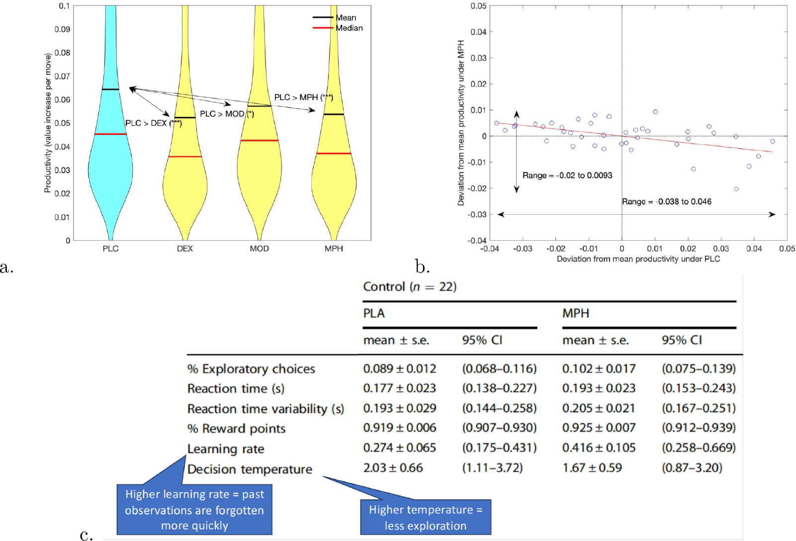
Figure 7. (a) Effect of dextro-amphetamine (DEX), modafinil (MOD), and methylphenidate (MPH) on productivity (PLC = placebo). Violin plots of all participant-trials. *** and * indicate significance at and , respectively. (b) Individual deviations in productivity from mean, methylphenidate (MPH) treatment against placebo (PLC); slope of regression line is significant at , corrected for estimation error in deviations; drop in range is significant at . (a) and (b) reproduced from Bowman et al. (2023). (c) Effects of MPH on choices in a probabilistic task, healthy controls (PLA = placebo). Extracted from Addicott et al. (2021, table 2).
(a) Effect of dextro-amphetamine (DEX), modafinil (MOD), and methylphenidate (MPH) on productivity (PLC = placebo). Violin plots of all participant-trials. *** and * indicate significance at p=0.001 and p=0.05, respectively. (b) Individual deviations in productivity from mean, methylphenidate (MPH) treatment against placebo (PLC); slope of regression line is significant at p=0.001, corrected for estimation error in deviations; drop in range is significant at p=10−4. (a) and (b) reproduced from Bowman et al. (2023). (c) Effects of MPH on choices in a probabilistic task, healthy controls (PLA = placebo). Extracted from Addicott et al. (2021, table 2).
Under methylphenidate, the reduction in performance was especially acute in participants who performed above average under placebo. See figure 7(b). Notice also that the productivity range narrowed under methylphenidate (): the drugs could be said to have caused some kind of “democratization.” A closer investigation revealed that above-average performers became more erratic. In particular, the value of the first knapsack filled became less predictive of the correct solution. In contrast, in previous research, the composition of the first knapsack was shown to be an important determinant of whether a participant would eventually find the solution (Murawski and Bossaerts, 2016).
The pharmacological evidence therefore suggests that drugs that target the motivational and attentional network of the brain (which is what methylphenidate, dextro-amphetamine, and modafinil do) reduce the quality of “thinking” or “creative effort.” In computationally hard tasks such as KP, it makes participants’ searches more erratic or “random.”
In contrast, in probabilistic tasks such as the multiarmed bandit problem, random search is optimal, so the drugs should not affect performance. There, methylphenidate has been shown to make participants forget more, but since the drug motivates, they explore more and end up collecting an insignificantly higher number of reward points than under placebo. See figure 7(c).
Summary and Conclusion
What are the lessons learned from the research reported here?
-
To understand human performance and effort, it is unproductive to think of NP-hard problems as if they were just a gambling task where beliefs are subjective (necessarily subjective since such problems always have a deterministic answer).
-
In NP-hard problems, opportunism trumps rationality, since it allows the decision-maker to get an informed answer more quickly even if this implies violations of choice consistency axioms.
-
As a consequence, humans perform significantly better than predicted by the trial-and-error method.
-
As a second consequence, there may not exist an expected utility function with which to represent human choices. This compromises traditional economic analysis.
-
Humans rarely optimize fully in NP-hard problems; their choices do appear to be in line with the theory of approximation complexity in the sense that performance and effort can be predicted from the approximation class of which the problem at hand is a member.
-
The search paths for solutions to NP-hard problems are extremely variable, both between humans and between times, suggesting that (i) it is virtually impossible to identify a limited set of “algorithms” or “heuristics” that humans use and (ii) communication should be used to improve decision-making.
-
Markets provide an effective way to enhance individuals’ performance in NP-hard problems; with the right design, markets become “oracles.” The evidence is in sharp contrast with the performance of markets in purely probabilistic settings, like guessing the composition of an urn of colored balls. There, bubbles and “mirages” regularly emerge.
-
Because there does not exist (yet?) a uniformly best way to solve NP-hard problems, one should refrain from “nudging” people to use a particular algorithm.
-
One day some of the classifications of NP-hard problems may become inconsequential from a computational point of view; nevertheless, the classifications should remain relevant to predict human performance and effort.
-
Difficulty metrics based on phase transitions in problem spaces or on particular solution algorithms prove useful to predict human (and nonhuman primate) performance and effort.
-
Human effort allocation does not appear to be determined ex ante; the data appear to support the conjecture that effort grows over time and stops when either a definite solution is found or the time required to find an improvement reaches a certain limit.
-
The proposed conjecture is consistent with neural activation early in a decision trial, as it does not correlate with proven ex ante metrics of difficulty; in particular, brain activity is not correlated with prima facie evidence that an instance is overconstrained.
-
“Smart drugs” merely motivate humans to work harder; they reduce economic performance (value attained) in optimization problems and significantly reduce productivity, especially for above-average performers. They also lead humans to resort to trial and error, an approach that has the same asymptotic performance as the brute-force algorithm (which is to list all possible solutions and pick the best one).
Some of these conclusions may be disturbing, such as the fourth one, which warns that choices may not be representable in terms of maximization of any utility function, the starting point of traditional economic analysis. This must be qualified. The heterogeneity that characterizes human approaches to solving computationally complex problems (point 6) implies flexibility: humans adjust their “algorithms” to the instances at hand. This then explains why, when presented with a limited set of instances, humans quickly adapt to the set and end up choosing based on a learned stimulus-response relationship. The responses are optimal, which then means that there exists a utility function that, if maximized, can represent their choices. See Ortega and Stocker (2016).
Still, when occasionally presented with a “catch trial” (an instance outside the set on which participants were trained), Ortega and Stocker (2016) documented that performance decreases dramatically. Such is the nature of NP-hard problems: even if only a detail of an instance is changed, a stimulus-response relation learned through reinforcement may perform miserably. The learned relation is not robust at all. The agent has to go back to “thinking,” applying “creative effort.”
Human choices can thus be predicted successfully on the basis of utility maximization as long as the context is confined. However, the context dependence reduces the scope of application of utility theory since the utility function that can be deployed to predict behavior in any setting depends on the instances that the agent happened to have been exposed to before and cannot be applied elsewhere. The utility function can no longer be considered a “primitive” of a decision problem.
Through a dialogue between experiments and theory, we have learned a lot about human attitudes toward computational complexity. It is worth re-emphasizing that this dialogue was necessarily loose, because the theory does not really categorize problems in terms of difficulty. NP-hard problems are thought to be harder than problems in P. Maybe one day this will prove to be wrong. Likewise, fully polynomial-time approximable problems (members of FPTAS) cannot really be considered to be easier than problems that cannot be approximated in polynomial time; at the time of this writing, they merely seem to be easier. That this perception matters to predict human performance and effort implies that the classifications of the theory of computational complexity will remain relevant even if one day someone proves that P = NP (point 9).
Where the dialogue between experiments and theory became tighter was in the study of instance complexity, whether based on phase transitions or on particular algorithms (point 10). Still, the link was not perfect because the instance complexity metrics were constructed from algorithms that guarantee the correct solution, yet the experiments clearly showed that humans rarely care to find the correct solution.
Markets appeared to be one way to harness the heterogeneity in solution approaches when participants are faced with computationally hard problems (point 7). One wonders whether markets could play an even more constructive role. Under indivisibilities, the core problem in economics, namely allocating a limited budget to a number of priced items, is NP-hard. Indeed, it is a variation on the KP optimization problem; see Gilboa et al. (2021). This raises an interesting issue. Since the difficulty of the budget problem depends on the prices and those prices are set in equilibrium—this, at least, is what most economists would claim—one wonders whether equilibrium prices would be selected such that the budget problem always becomes easy. It would be wonderful to obtain such a result and test it in the laboratory. A rereading of Hayek (1945) suggests that he conjectured that the answer is yes. That is far from obvious since equilibrium prices may not even exist because of indivisibilities, as shown in, for example, Henry (1970).
The opposite may be true: to ensure equilibration, markets may select prices that cause agents’ budget allocation decisions to become so complex that many agents stop optimizing. In the language of the theory, market prices will be such that agents are confronted with instances of the budget allocation problem where the optima reside in the phase transition region. Only agents willing to put in substantial effort will end up maximizing utility. Others will choose differently, and suboptimally. Evidence has recently emerged that this is exactly what happens, even when equilibrium exists. See Bossaerts et al. (2026).
The consequences are disturbing. Anxiety has recently increased in modern societies (e.g., Goodwin et al., 2020). One way markets could cause anxiety is by making budget allocation instances hard: even if substantial effort is applied, the agent is still not sure whether she chooses in the best way. The recent rise in anxiety has coincided with an increased use of market-based solutions to solve societies’ problems, such as transportation (airline deregulation, railway privatization), medical care (healthcare marketplaces), education (higher education loan programs), and climate change (carbon markets). One wonders whether there is a link?
References
- Addicott, M. A., Pearson, J. M., Schechter, J. C., Sapyta, J. J., Weiss, M. D., & Kollins, S. H. (2021). Attention-deficit/hyperactivity disorder and the explore/exploit trade-off. Neuropsychopharmacology, 46(3), 614–621.
- Arora, S., & Barak, B. (2009). Computational complexity: A modern approach. Cambridge University Press.
- Attneave, F. (1954). Some informational aspects of visual perception. Psychological Review, 61(3), 183.
- Azeredo da Silveira, R., & Woodford, M. (2019). Noisy memory and over-reaction to news. AEA Papers and Proceedings, 109, 557–561.
- Banovetz, J., & Oprea, R. (2023). Complexity and procedural choice. American Economic Journal: Microeconomics, 15(2), 384–413. https://doi.org/10.1257/mic.20210032
- Barlow, H. B. (1961). Possible principles underlying the transformation of sensory messages. Sensory Communication, 1(1), 217–233.
- Berrada, T., Bossaerts, P., & Ugazio, G. (2024). Investments and asset pricing in a world of satisficing agents (Research Paper 24–05). Swiss Finance Institute.
- Best, B. J. (2006). Cognitive approaches to the traveling salesperson problem: Perceptual complexity that produces computational simplicity. In AAAI Spring Symposium: Between a Rock and a Hard Place: Cognitive Science Principles Meet AI-Hard Problems (pp. 11–16). Association for the Advancement of Artificial Intelligence.
- Bossaerts, P., Bowman, E., Fattinger, F., Huang, H., Lee, M., Murawski, C., Suthakar, A., Tang, S., & Yadav, N. (2024). Resource allocation, computational complexity, and market design. Journal of Behavioral and Experimental Finance, 42, 100906.
- Bossaerts, P., Ioannidis, K., Woods, R., & Yadav, N. (2026). How computational complexity can restore general equilibrium in markets with indivisible goods (SSRN 6002716). https://papers.ssrn.com/sol3/papers.cfm?abstract_id=6002716
- Bossaerts, P., Yadav, N., & Murawski, C. (2019). Uncertainty and computational complexity. Philosophical Transactions of the Royal Society B, 374(1766), 20180138.
- Bowman, E., Coghill, D., Murawski, C., & Bossaerts, P. (2023). Not so smart? “Smart” drugs increase the level but decrease the quality of cognitive effort. Science Advances, 9(24), eadd4165.
- Bowman, E., Feng, B., Murawski, C., & Bossaerts, P. (2020). Surveying the use of pharmaceutical cognitive enhancers in the Australian financial services industry (SSRN 3661966). https://papers.ssrn.com/sol3/papers.cfm?abstract_id=3661966
- Brock, W. A., & Dechert, W. D. (1991). Non-linear dynamical systems: Instability and chaos in economics. Handbook of Mathematical Economics, 4, 2209–2235.
- Camara, M. K. (2022). Computationally tractable choice. In Proceedings of the 23rd ACM Conference on Economics and Computation (pp. 28ff). Association for Computing Machinery.
- Camerer, C., & Weigelt, K. (1991). Information mirages in experimental asset markets. Journal of Business, 64(4), 463–493.
- Caplin, A., Dean, M., & Martin, D. (2011). Search and satisficing. American Economic Review, 101(7), 2899–2922.
- Cook, S. A. (1983). An overview of computational complexity. Communications of the ACM, 26(6), 400–408.
- Corgnet, B., Deck, C., DeSantis, M., Hampton, K., & Kimbrough, E. O. (2023). When do security markets aggregate dispersed information? Management Science, 69(6), 3697–3729.
- Daw, N. D., O’Doherty, J. P., Dayan, P., Seymour, B., & Dolan, R. J. (2006). Cortical substrates for exploratory decisions in humans. Nature, 441(7095), 876–879. https://doi.org/10.1038/nature0476610.1038/nature04766
- Echenique, F., Golovin, D., & Wierman, A. (2011). A revealed preference approach to computational complexity in economics. In Proceedings of the 12th ACM conference on Electronic Commerce (pp. 101–110). Association for Computing Machinery.
- Eisenführ, F., Weber, M., & Langer, T. (2010). Rational decision making. Springer.
- Enke, B. (2024). The cognitive turn in behavioral economics. Harvard University.
- Enke, B., & Graeber, T. (2023). Cognitive uncertainty. The Quarterly Journal of Economics, 138(4), 2021–2067.
- Fattinger, F. (2021). Trading complex risks (SSRN 3086358). https://papers.ssrn.com/sol3/papers.cfm?abstract_id=3086358
- Franco, J. P., Bossaerts, P., & Murawski, C. (2024). The neural dynamics associated with computational complexity. PLOS Computational Biology, 20(9), e1012447. https://doi.org/10.1371/journal.pcbi.1012447
- Franco, J. P., Doroc, K., Yadav, N., Bossaerts, P., & Murawski, C. (2022). Task-independent metrics of computational hardness predict human cognitive performance. Scientific Reports, 12(1), 12914.
- Franco, J. P., Yadav, N., Bossaerts, P., & Murawski, C. (2021). Generic properties of a computational task predict human effort and performance. Journal of Mathematical Psychology, 104, 102592.
- Frydman, C., & Jin, L. J. (2022). Efficient coding and risky choice. The Quarterly Journal of Economics, 137(1), 161–213.
- Gent, I. P., & Walsh, T. (1996). The TSP phase transition. Artificial Intelligence, 88(1–2), 349–358.
- Gigerenzer, G., & Selten, R. (2002). Bounded rationality: The adaptive toolbox. MIT Press.
- Gilboa, I., Postlewaite, A., & Schmeidler, D. (2021). The complexity of the consumer problem. Research in Economics, 75(1), 96–103.
- Glimcher, P. W. (2022). Efficiently irrational: Deciphering the riddle of human choice. Trends in Cognitive Sciences, 26(8), 669–687.
- Glimcher, P. W., & Tymula, A. A. (2023). Expected subjective value theory (ESVT): A representation of decision under risk and certainty. Journal of Economic Behavior & Organization, 207, 110–128.
- Goodwin, R. D., Weinberger, A. H., Kim, J. H., Wu, M., & Galea, S. (2020). Trends in anxiety among adults in the United States, 2008–2018: Rapid increases among young adults. Journal of Psychiatric Research, 130, 441–446.
- Hanneke, S. (2016). The optimal sample complexity of PAC learning. The Journal of Machine Learning Research, 17(1), 1319–1333.
- Hayek, F. A. (1945). The use of knowledge in society. The American Economic Review, 35(4), 519–530.
- Henry, C. (1970). Indivisibilités dans une économie d’échanges. Econometrica: Journal of the Econometric Society, 38(3), 542–558.
- Hong, T., & Stauffer, W. R. (2023). Computational complexity drives sustained deliberation. Nature Neuroscience, 26, 850–857.
- Karp, R. M. (1972). Reducibility among combinatorial problems. In Complexity of Computer Computations (pp. 85–103). Springer.
- Kendall, C., & Oprea, R. (2024). On the complexity of forming mental models. Quantitative Economics, 15(1), 175–211.
- Lieder, F., & Griffiths, T. L. (2020). Resource-rational analysis: Understanding human cognition as the optimal use of limited computational resources. Behavioral and Brain Sciences, 43, e1.
- Louie, K., Khaw, M. W., & Glimcher, P. W. (2013). Normalization is a general neural mechanism for context-dependent decision making. Proceedings of the National Academy of Sciences, 110(15), 6139–6144.
- Meloso, D., Copic, J., & Bossaerts, P. (2009). Promoting intellectual discovery: Patents versus markets. Science, 323(5919), 1335–1339.
- Monasson, R., Zecchina, R., Kirkpatrick, S., Selman, B., Troyansky, L., Lhomond, R., Watson, T. J., & Heights, Y. (1999). Determining computational complexity from characteristic ‘phase transitions.’. Nature, 400(6740), 133–137. https://doi.org/10.1038/22055
- Murawski, C., & Bossaerts, P. (2016). How humans solve complex problems: The case of the knapsack problem. Scientific Reports, 6, 34851.
- Newell, A., & Simon, H. A. (1972). Human problem solving (Vol. 104). Prentice Hall.
- Oprea, R. (2020). What makes a rule complex? American Economic Review, 110(12), 3913–3951.
- Oprea, R. (2024). Complexity and its measurement. University of California Santa Barbara.
- Ortega, P. A., & Stocker, A. A. (2016). Human decision-making under limited time. Advances in Neural Information Processing Systems, 29.
- Page, L. (2022). Optimally irrational: The good reasons we behave the way we do. Cambridge University Press.
- Page, L., & Siemroth, C. (2021). How much information is incorporated into financial asset prices? Experimental evidence. The Review of Financial Studies, 34(9), 4412–4449.
- Pape, T., Kavadias, S., & Sommer, S. C. (2020). Decision bias in project selection: Experimental evidence from the knapsack problem (SSRN 3448676). https://papers.ssrn.com/sol3/papers.cfm?abstract_id=3448676
- Payzan-LeNestour, E., Dunne, S., Bossaerts, P., & O’Doherty, J. P. (2013). The neural representation of unexpected uncertainty during value-based decision making. Neuron, 79(1), 191–201.
- Payzan-LeNestour, E., & Woodford, M. (2022). Outlier blindness: A neurobiological foundation for neglect of financial risk. Journal of Financial Economics, 143(3), 1316–1343.
- Polanía, R., Woodford, M., & Ruff, C. C. (2019). Efficient coding of subjective value. Nature Neuroscience, 22(1), 134–142.
- Preuschoff, K., Quartz, S. R., & Bossaerts, P. (2008). Human insula activation reflects risk prediction errors as well as risk. Journal of Neuroscience, 28(11), 2745–2752.
- Reutskaja, E., Lindner, A., Nagel, R., Andersen, R. A., & Camerer, C. F. (2018). Choice overload reduces neural signatures of choice set value in dorsal striatum and anterior cingulate cortex. Nature Human Behaviour, 2(12), 925–935.
- Rich, P., Blokpoel, M., de Haan, R., & van Rooij, I. (2020). How intractability spans the cognitive and evolutionary levels of explanation. Topics in Cognitive Science, 12(4), 1382–1402. https://doi.org/https://doi.org/10.1111/tops.12506
- Rissanen, J. (1987). Stochastic complexity. Journal of the Royal Statistical Society: Series B (Methodological), 49(3), 223–239.
- Sahni, S. (1975). Approximate algorithms for the 0/1 knapsack problem. Journal of the ACM, 22(1), 115–124.
- Sanjurjo, A. (2015). Search, memory, and choice error: An experiment. PLoS One, 10(6), e0126508.
- Sanjurjo, A. (2023). Space complexity in choice (SSRN working paper 4580158). http://dx.doi.org/10.2139/ssrn.4580158
- Simon, H. A. (1955). A behavioral model of rational choice. The Quarterly Journal of Economics, 69(1), 99–118.
- Tenbrink, T., & Wiener, J. (2009). The verbalization of multiple strategies in a variant of the traveling salesperson problem. Cognitive Processing, 10, 143–161.
- Tversky, A., & Kahneman, D. (1974). Judgment under uncertainty: Heuristics and biases. Science, 185(4157), 1124–1131.
- Vieider, F. M. (2024). Decisions under uncertainty as Bayesian inference on choice options. Management Science, 70(12), 9014–9030.
- Wilson, R. C., Nassar, M. R., & Gold, J. I. (2013). A mixture of delta-rules approximation to Bayesian inference in change-point problems. PLoS Computational Biology, 9(7), e1003150.
- Yadav, N., Hsu, A., Franco, J. P., Bossaerts, P., & Murawski, C. (2024). How well could and do humans approximate optimality? [Manuscript submitted for publication].
- Yadav, N., Murawski, C., Sardina, S., & Bossaerts, P. (2020). Is hardness inherent in computational problems? Performance of human and electronic computers on random instances of the 0-1 knapsack problem. In ECAI 2020 (pp. 498–505). IOS Press.
- Yamada, H., Louie, K., Tymula, A., & Glimcher, P. W. (2018). Free choice shapes normalized value signals in medial orbitofrontal cortex. Nature Communications, 9(1), 162.
Figures
Figure 1. (a) Map of the European Union, downloaded from https://european-union.europa.eu/. The graph coloring task consists of finding whether member countries could be assigned colors so that no contiguous countries display the same color without using more than a limited number of colors, say four. In the map, more than 10 colors were used. (b) Which bin, if filled to capacity with a selection of the items depicted next to them, maximizes value? The greedy algorithm generates the wrong answer and hence does not maximize utility, even if it has good approximation properties in general. (c) Graphical interface of the knapsack problem optimization tasks used in experiments. Items from the right are to be moved into the knapsack to the left to maximize total value (in euros) without violating the capacity (expressed in kg). Reproduced from Bossaerts et al. (2024).
(a) Map of the European Union, downloaded from https://european-union.europa.eu/. The graph coloring task consists of finding whether member countries could be assigned colors so that no contiguous countries display the same color without using more than a limited number of colors, say four. In the map, more than 10 colors were used. (b) Which bin, if filled to capacity with a selection of the items depicted next to them, maximizes value? The greedy algorithm generates the wrong answer and hence does not maximize utility, even if it has good approximation properties in general. (c) Graphical interface of the knapsack problem optimization tasks used in experiments. Items from the right are to be moved into the knapsack to the left to maximize total value (in euros) without violating the capacity (expressed in kg). Reproduced from Bossaerts et al. (2024).
Figure 2. (a) Feasible search paths in item/value space for a knapsack problem (KP) optimization problem with N = 10 items; horizontal: value attained; vertical: distance from the optimal knapsack, in number of items. Participants start with zero items, at which point the value is zero and they are seven items away from the optimum. Each participant-trial (40 in total) is depicted with a different color; large dots indicate final positions. More than 40% of feasible paths are colored, suggesting that search approaches were extremely heterogeneous. (b) Performance, per instance (a) and per participant (b); performance is measured as the fraction of instances where the optimum was found. (a) and (b) reproduced from Murawski and Bossaerts (2016). Evolution of trade prices in a market for a security that paid the true optimal value of a KP optimization instance; five instances are shown. A solid vertical line depicts the optimal value; dotted lines denote the second- and third-best solution values, and for the rightmost instance (the most difficult one; see section 6 on how to measure instance difficulty), up to the fifth best solution. Reproduced from Bossaerts et al. (2024).
(a) Feasible search paths in item/value space for a knapsack problem (KP) optimization problem with N = 10 items; horizontal: value attained; vertical: distance from the optimal knapsack, in number of items. Participants start with zero items, at which point the value is zero and they are seven items away from the optimum. Each participant-trial (40 in total) is depicted with a different color; large dots indicate final positions. More than 40% of feasible paths are colored, suggesting that search approaches were extremely heterogeneous. (b) Performance, per instance (a) and per participant (b); performance is measured as the fraction of instances where the optimum was found. (a) and (b) reproduced from Murawski and Bossaerts (2016). Evolution of trade prices in a market for a security that paid the true optimal value of a KP optimization instance; five instances are shown. A solid vertical line depicts the optimal value; dotted lines denote the second- and third-best solution values, and for the rightmost instance (the most difficult one; see section 6 on how to measure instance difficulty), up to the fifth best solution. Reproduced from Bossaerts et al. (2024).
Figure 3. (a) Visual representation of instances of three NP-complete decision problems: 3-SAT (left), traveling salesperson problem (TSP; middle), and knapsack problem (KP; right). (b) Boxplots of human performance (a) and effort (b) in the three problems (effort for the KP is not shown since it was not self-paced); instances are stratified in terms of typical case complexity (TCC; whether in or outside the phase transition) and solvability (“satisfiability:” red indicates that the correct answer was “yes;” otherwise green color is used). (a) and (b) reproduced from Franco et al. (2022). (c) Time needed to increase value in the KP optimization problem or declare that an optimum has been reached, as a function of the log-ratio of normalized capacity c and normalized values p, for humans (a) and machines (electronic computer) (b). Humans solved instances of 10 items, not always correctly; a computer program (MiniZinc) solved instances of 50 items, always correctly. A phase transition is discernible, where the log-ratio is close to and below zero. Reproduced from Yadav et al. (2020).
(a) Visual representation of instances of three NP-complete decision problems: 3-SAT (left), traveling salesperson problem (TSP; middle), and knapsack problem (KP; right). (b) Boxplots of human performance (a) and effort (b) in the three problems (effort for the KP is not shown since it was not self-paced); instances are stratified in terms of typical case complexity (TCC; whether in or outside the phase transition) and solvability (“satisfiability:” red indicates that the correct answer was “yes;” otherwise green color is used). (a) and (b) reproduced from Franco et al. (2022). (c) Time needed to increase value in the KP optimization problem or declare that an optimum has been reached, as a function of the log-ratio of normalized capacity c and normalized values p, for humans (a) and machines (electronic computer) (b). Humans solved instances of 10 items, not always correctly; a computer program (MiniZinc) solved instances of 50 items, always correctly. A phase transition is discernible, where the log-ratio is close to and below zero. Reproduced from Yadav et al. (2020).
Figure 4. (a) Three graph problems: random traveling salesperson problem (RTSP), where the shortest feasible path is to be found connecting all nodes without visiting any node twice; Euclidean traveling salesperson problem (ETSP), like RTSP, but where distances (indicated with ⋯) satisfy Euclidean restrictions; and weighted cost shortest path problem (WCSPP), where the path with the shortest distance has to be found between a Start and End point while costs from feasible transits remain within a limit. (b) Kernel densities of human performance [R(x, w)] in the three problems. (c) Effort in the three problems in terms of the number of mouse clicks (left) or time (right). (d) Expected average error [] from randomly choosing feasible paths is higher in RTSP than in ETSP despite an equal number of feasible paths. All panels reproduced from Yadav et al. (2024).
(a) Three graph problems: random traveling salesperson problem (RTSP), where the shortest feasible path is to be found connecting all nodes without visiting any node twice; Euclidean traveling salesperson problem (ETSP), like RTSP, but where distances (indicated with ⋯) satisfy Euclidean restrictions; and weighted cost shortest path problem (WCSPP), where the path with the shortest distance has to be found between a Start and End point while costs from feasible transits remain within a limit. (b) Kernel densities of human performance [R(x, w)] in the three problems. (c) Effort in the three problems in terms of the number of mouse clicks (left) or time (right). (d) Expected average error [1−1/ R(x,w)] from randomly choosing feasible paths is higher in RTSP than in ETSP despite an equal number of feasible paths. All panels reproduced from Yadav et al. (2024).
Figure 5. (a) Individual performance (percentage instances solved correctly) in the knapsack problem (KP) optimization problem with items as a function of Sahni-k; 20 participants, 16 instances. Reproduced from Murawski and Bossaerts (2016). (b) Performance of an algorithm based on market prices of binary options that pay 1 if the corresponding item is in the optimal solution and 0 otherwise (blue), against performance of individual traders in the marketplace (red), as a function of Sahni-k. Humans do significantly better than individuals on average; between 18 and 20 participants per marketplace. Reproduced from Bossaerts et al. (2024). (c) Individuals’ performance and effort in KP (optimization), as a function of typical case complexity; 20 participants, 18 instances of N = 6 items each. Reproduced from Franco et al. (2021).
(a) Individual performance (percentage instances solved correctly) in the knapsack problem (KP) optimization problem with N=10,12 items as a function of Sahni-k; 20 participants, 16 instances. Reproduced from Murawski and Bossaerts (2016). (b) Performance of an algorithm based on market prices of binary options that pay 1 if the corresponding item is in the optimal solution and 0 otherwise (blue), against performance of individual traders in the marketplace (red), as a function of Sahni-k. Humans do significantly better than individuals on average; between 18 and 20 participants per marketplace. Reproduced from Bossaerts et al. (2024). (c) Individuals’ performance and effort in KP (optimization), as a function of typical case complexity; 20 participants, 18 instances of N = 6 items each. Reproduced from Franco et al. (2021).
Figure 6. (a) Brain regions of interest (ROI): insula [only anterior part (AI) is of interest]; cingulate cortex [only dorsal–upper–anterior part (dACC) is of interest]; angular gyrus (AG)/intraparietal sulcus (IPS). (b) Time courses and differences relative to start time of a trial but adjusted for a 5 second fMRI signal delay; average across participant-trials extracted using random-effects general linear modeling and stratified by solvability (satisfiability) and typical case complexity (TCC). High TCC = target value is in the phase transition; low TCC = target value is outside phase transition, and hence, the instance is either underconstrained (and hence solvable) or overconstrained (and hence unsolvable). Red asterisks indicate significant differences at . Significance levels in grey-colored epochs in the TCC plots are suggestive only because they do not correct for the fact that the ROIs were extracted from whole-brain corrected neural activation difference for the shown contrast (TCC) during the epoch indicated. All panels reproduced from Franco et al. (2024).
(a) Brain regions of interest (ROI): insula [only anterior part (AI) is of interest]; cingulate cortex [only dorsal–upper–anterior part (dACC) is of interest]; angular gyrus (AG)/intraparietal sulcus (IPS). (b) Time courses and differences relative to start time of a trial but adjusted for a 5 second fMRI signal delay; average across participant-trials extracted using random-effects general linear modeling and stratified by solvability (satisfiability) and typical case complexity (TCC). High TCC = target value is in the phase transition; low TCC = target value is outside phase transition, and hence, the instance is either underconstrained (and hence solvable) or overconstrained (and hence unsolvable). Red asterisks indicate significant differences at p=0.05. Significance levels in grey-colored epochs in the TCC plots are suggestive only because they do not correct for the fact that the ROIs were extracted from whole-brain corrected neural activation difference for the shown contrast (TCC) during the epoch indicated. All panels reproduced from Franco et al. (2024).
Figure 7. (a) Effect of dextro-amphetamine (DEX), modafinil (MOD), and methylphenidate (MPH) on productivity (PLC = placebo). Violin plots of all participant-trials. *** and * indicate significance at and , respectively. (b) Individual deviations in productivity from mean, methylphenidate (MPH) treatment against placebo (PLC); slope of regression line is significant at , corrected for estimation error in deviations; drop in range is significant at . (a) and (b) reproduced from Bowman et al. (2023). (c) Effects of MPH on choices in a probabilistic task, healthy controls (PLA = placebo). Extracted from Addicott et al. (2021, table 2).
(a) Effect of dextro-amphetamine (DEX), modafinil (MOD), and methylphenidate (MPH) on productivity (PLC = placebo). Violin plots of all participant-trials. *** and * indicate significance at p=0.001 and p=0.05, respectively. (b) Individual deviations in productivity from mean, methylphenidate (MPH) treatment against placebo (PLC); slope of regression line is significant at p=0.001, corrected for estimation error in deviations; drop in range is significant at p=10−4. (a) and (b) reproduced from Bowman et al. (2023). (c) Effects of MPH on choices in a probabilistic task, healthy controls (PLA = placebo). Extracted from Addicott et al. (2021, table 2).